
Working Paper Series
Caution: do not cross!
Capital buffers and lending
in Covid-19 times
Cyril Couaillier, Marco Lo Duca,
Alessio Reghezza, Costanza Rodriguez d’Acri
Disclaimer: This paper should not be reported as representing the views of the European Central Bank
(ECB). The views expressed are those of the authors and do not necessarily reflect those of the ECB.
No 2644 / February 2022
Abstract
While regulatory capital buffers are expected to be drawn to absorb losses and meet credit
demand during crises, this paper shows that banks were unwilling to do so during the
pandemic. To the contrary, banks engaged in forms of pro-cyclical behaviour to preserve
capital ratios. By employing granular data from the credit register of the European
System of Central Banks, we isolate credit supply effects and find that banks with little
headroom above regulatory buffers reduced their lending relative to other banks, also
when controlling for a broad range of pandemic support measures. Firms’ inability to
reallocate their credit needs to less constrained banks had real economic effects, as their
headcount went down, although state guarantee schemes acted as partial mitigants. These
findings point to some unintended effects of the capital framework which may create
incentives for pro-cyclical behaviour by banks during downturns. They also shed light
on the interactions between fiscal and prudential policies which took place during the
pandemic.
JEL classification: E61; G01; G18; G21
Keywords: Coronavirus; Macroprudential policy; MDA distance; Bank lending; Buffer
usability; Credit register
ECB Working Paper Series No 2644 / February 2022
1
Non-technical summary
The Basel III capital framework provides the foundations for the prudential supervision
of banks (BCBS, 2011). Its goal is to reduce the pro-cyclical effects of the banking system
on the economic cycle, namely to limit bank risk-taking and excessive credit growth in
good times and credit supply contractions during periods of economic distress. To this
aim, the framework envisages that bank capital is built up during economic upturns and
then employed to absorb losses and meet credit demand during economic downturns and
crises. The deep economic recession, the economic uncertainty, the prospect of serious
deterioration in bank asset quality and profitability caused by the Covid-19 pandemic
provided a first test of the capital framework. By analysing euro area banks’ behaviour
during the pandemic, this paper investigates banks’ willingness (or unwillingness) to make
use of capital buffers, as envisaged by Basel III.
Banks in the euro area entered the Covid-19 pandemic with relatively strong capital
ratios (Enria, 2020), however, most of this capital was held in the form of prudential
regulatory buffers. These buffers sit on top of minimum capital requirements and con-
stitute the combined buffer requirement (CBR). The CBR abets banks to absorb losses
while continuing to provide key financial services during distressed periods, thus mitigat-
ing negative externalities related to credit rationing and asset fire sales that could harm
the economy (Acharya et al. 2017). However, banks’ willingness or ability to draw down
the CBR may be limited by a several factors, including limitations to distributions (ac-
cording to the Maximum Distributable Amount – MDA – mechanism), market pressure
and stigma. Ultimately, impediments to the use of buffers can negatively affect lending
supply to the real economy when most needed, thereby causing pro-cyclical amplification.
In this paper, we investigate empirically whether banks closer to the MDA trigger take
adjustment actions curtailing their lending to NFCs during the pandemic in comparison
to banks further away from the MDA. This research question is of primary importance
for policy makers as it points to possible unintended distortions in the capital framework
and possible pro-cyclical effects during downturns (Behn et al., 2020).
ECB Working Paper Series No 2644 / February 2022
2
We employ loan-level data to exploit multiple bank relationships, thus controlling for
credit demand effects (Khwaja and Mian, 2008). We also match our datasets with bank-
and loan-level information on banks’ features including reliance on central bank funding,
payment moratoria and government guaranteed loans. In this way we isolate credit supply
effects triggered by the proximity to the MDA from other bank specific features and from
pandemic-related support measures which also have an impact on lending. We apply
sample matching strategies to convey robust results and ensure that results are not driven
by other possible explanations.
The results of our analysis show that proximity to the MDA trigger results in lower
lending to NFCs. Specifically, we find that proximity to the MDA reduces lending by
about 3.5% to NFCs during the pandemic. We also find that lower lending from banks
in proximity of the MDA trigger resulted in credit constraints to firms exposed to these
banks as lost loans were not fully replaced. In particular, firms that prior to the pandemic
received most of their borrowing from banks closer to the MDA trigger experienced about
2.5% lower borrowing during the pandemic in comparison to firms that borrowed mostly
from other banks. We document that this lack of perfect credit substitution led to firms
cutting down their headcounts by close to 1% in comparison to other firms. Finally, we
show that government guarantees ameliorated the negative effect caused by proximity to
the MDA trigger as firms receiving loans covered by government schemes counter off the
lending impairments caused by banks in proximity of the MDA trigger.
Beyond contributing to different strands of the academic literature on banking, these
findings inform the current debate on the appropriateness of the capital buffer framework
and support discussions on how to improve its design. They also shed some light on the
fiscal and prudential policies’ interactions which took place during the pandemic.
ECB Working Paper Series No 2644 / February 2022
3

1 Introduction
The Basel III capital framework provides the foundations for the prudential supervision
of banks (BCBS, 2011). Its goal is to reduce the pro-cyclical effects of the banking system
on the economic cycle, namely to limit bank risk-taking and excessive credit growth in
good times and credit supply contractions during periods of economic distress. To this
aim, the framework envisages that bank capital is built up during economic upturns and
then employed (i.e. by allowing temporary declines in capital ratios) to absorb losses and
meet credit demand during economic downturns and crises. The deep economic recession
and the economic uncertainty caused by the Covid-19 pandemic provided a first test of
the Basel III capital framework. By analysing euro area banks’ behaviour during the
pandemic, this paper investigates banks’ willingness (or unwillingness) to make use of
capital buffers, as envisaged by Basel III.
The rapid spread of Covid-19 worldwide confronted policymakers not only with a
major public health problem but also with the prospect of a serious economic and financial
crisis. While prompt and forceful policy actions assuaged the worst economic effects of
the pandemic,
2
restrictions on personal mobility and nonessential business operations
strongly affected business profits, causing a surge in liquidity needs. At the same time,
those containment measures caused a major global economic contraction. As such, banks
faced simultaneously a surge in credit demand and the prospect of serious deterioration in
asset quality and profitability. Therefore, in this paper we exploit the exogenous economic
shock caused the Covid-19 pandemic to assess banks’ behaviour and their willingness to
use regulatory capital in periods of severe economic distress.
Banks in the euro area entered the Covid-19 pandemic with on average strong capital
ratios (Enria, 2020). Most of this capital was raised to meet capital requirements (Figure
1): the minimum requirements that banks must meet at all times and the combined
2
Monetary policy ensured accommodative financing conditions overall and for banks. Fiscal policy
provided support to household and firms via tax credit, direct transfers, job support schemes, debt
moratoria and loan guarantees (ECB, 2020). Prudential authorities also adopted a number of measures
to allow banks to operate with more flexibility during the pandemic (SSM, March 2020).
ECB Working Paper Series No 2644 / February 2022
4

buffer requirements (thereafter CBR). The latter capital buffers sit on top of minimum
capital requirements and, in the European framework, consist of the capital conservation
buffer (CCoB), counter cyclical buffer (CCyB), systemic risk buffer (SyRB) and buffers for
systemically important banks (Figure 2).
3
The CBR abets banks to absorb losses while
continuing to provide key financial services during distressed periods, thus mitigating
negative externalities related to credit rationing and asset fire sales that could harm the
economy (Acharya et al. 2017). Indeed, whereas minimum capital requirements must be
met on an ongoing basis, the CBR can, in principle, be drawn down when needed during
severe downturns or financial crises. Consequently, capital ratios may dip into the CBR in
order to: (i) cushion the materialisation of losses (i.e. the numerator of the capital ratio)
and; (ii) allow for increases in risk-weighted assets (i.e. the denominator of the capital
ratio).
[Insert Figure 1 Here]
[Insert Figure 2 Here]
While prudential authorities made clear at the beginning of the pandemic that banks
were expected to use the CBR in case of need (Enria, 2020; BIS, 2020; FSB, 2020), banks’
willingness or ability to draw down buffers may be limited by a number of factors. First,
dipping into the CBR triggers restrictions on dividend distributions, bonuses and coupon
payments according to the Maximum Distributable Amount (MDA) mechanism (Svoronos
and Vrbaski, 2020). Although European supervisors encouraged the suspension of divi-
dend payouts during the Covid-19 pandemic, banks may still want to avoid breaching the
MDA trigger in order to distribute dividends as soon as the ban is lifted. Second, dipping
into the CBR could provide a negative signal to the market in respect to bank’s solvency
(Drehmann et al., 2020; Baker and Wurgler, 2015). This can lead to higher funding costs
and/or have negative implications for bank credit ratings (Claessens et al., 2018). Third,
banks’ willingness to draw down buffers depends on the expected reaction of supervisory
3
These are buffers for Other Systemically Important Intermediaries (O-SIIs), which are systemic do-
mestic banks, and for Globally Systemically Important Banks (G-SIBs)
ECB Working Paper Series No 2644 / February 2022
5

authorities (Borio et al., 2020). If banks expect heightened scrutiny because of a breach
of the CBR (EBA, 2021), it is unlikely that banks will make use of it.
4
Additionally,
banks might be uncertain about the time they will be given to replenish capital buffers.
Such concerns may be more relevant when profitability is low or access to capital markets
is constrained. Finally, other regulatory requirements such as the leverage ratio or the
Minimum Requirement for own funds and Eligible Liabilities (MREL) constrain the us-
ability of buffers if they are more binding than risk-based requirements (BoP, 2020). For
the above reasons, banks tend to keep capital targets above the CBR (Couaillier, 2020;
Behn et al., 2020) by holding excess capital (or management buffers).
5
Bank unwillingness to draw down buffers can negatively affect lending supply to the
real economy when most needed. In this paper, we investigate empirically whether banks
closer to the MDA trigger take adjustment actions to preserve capital ratios, curtailing
their lending to non-financial corporations (NFCs) during the pandemic in comparison to
banks further away from the MDA trigger. This research question is of primary impor-
tance for policy makers as it points to possible unintended effects of the capital framework
and possible pro-cyclical behaviour of banks during downturns (Behn et al., 2020).
Our analysis offers a comprehensive assessment of the effect of proximity to the MDA
trigger on bank credit supply adjustments following the pandemic outbreak. Specifically,
we answer the following questions: Did banks closer to the MDA trigger curtail their lend-
ing in comparison to banks further away from it? Did firms most exposed to these banks
experience a contraction in credit? Did government guaranteed schemes ameliorated the
negative effect coming from banks’ proximity to the MDA trigger? We rely on granular
loan-level data to address these questions.
Several empirical challenges must be overcome to estimate the effect of proximity to
4
When approaching the MDA trigger, a bank must inform the supervisor of a Capital Conservation
Plan describing how it intends to replenish its buffer. Should the supervisor disagree with the plan, it
can require the institution to increase capital in a specified period and lower the MDA (Article 142 of
CRD IV).
5
Bank management buffers (or excess capital) support banks’ credit ratings and business model strate-
gies, but, more importantly for this paper, they insulate banks from the supervisory interventions which
are triggered when regulatory capital requirements are breached.
ECB Working Paper Series No 2644 / February 2022
6
the MDA trigger on lending behaviour during the Covid-19 pandemic. First, it requires
accounting for the large surge in credit demand from firms for emergency liquidity needs
during the pandemic. In this respect, we rely on granular loan-level data taken from the
analytical credit register (AnaCredit) of the European System of Central Banks. In partic-
ular, we exploit a difference-in-differences (DiD) framework with multiple bank relation-
ships and firm fixed effects (Khwaja and Mian, 2008) as well as single-bank relationship
via the inclusion of industry-location-size fixed effects to control for the heterogeneity
in credit demand across firms (Degryse et al., 2019). Second, it necessitates isolating
bank credit supply from pandemic-related measures: most notably, government guaran-
tee and moratoria schemes. Government guarantees on new loans helped firms obtaining
bank loans to roll over liquidity and working capital needs while debt service morato-
ria have also been widely introduced to mitigate the liquidity concerns of households
and firms. To control for the confounding effect of these measures on bank lending, we
match AnaCredit with bank-firm level information on payment moratoria and govern-
ment guarantees. Third, we account for monetary and prudential measures by including
unconventional monetary policy (TLTRO III) and the ECB recommendation on dividend
distribution in our empirical strategy. Altavilla et al. (2020) show that in the absence
of TLTRO III lending to firms would have been 3 percentage points lower. Additionally,
Martinez-Miera and Vegas (2021) find that banks extended significantly more credit to
non-financial corporations after the entry into force of the recommendation. We also use
propensity score matching (PSM) estimations to select banks that share similar charac-
teristics but differing in terms of their proximity to the MDA trigger, thereby ensuring
that results are not endogenous, i.e. driven by weaker balance sheets for banks closer to
the MDA trigger point.
To preview our findings, proximity to the MDA trigger results in lower lending to
NFCs. Specifically, we find that proximity to the MDA reduces lending by about 3.5%
to NFCs during the pandemic. We also find that lower lending from banks in proximity
of the MDA trigger resulted in credit constraints for firms exposed to these banks as lost
loans were not fully replaced. In particular, firms that prior to the pandemic received
ECB Working Paper Series No 2644 / February 2022
7

most of their borrowing from banks closer to the MDA trigger experienced about 2.5%
lower borrowing during the pandemic in comparison to firms that borrowed mostly from
other banks. We document that this lack of perfect credit substitution led to firms cutting
down their headcounts by close to 1% in comparison to other firms. Finally, we show that
government guarantees ameliorated the negative effect caused by the proximity to the
MDA trigger. In particular, firms receiving loans covered by government schemes counter
off the lending impairments caused by banks in proximity of the MDA trigger.
Our paper provides a solid contribution to the extant literature in several respects.
First, we add to the long-standing empirical literature on bank capitalisation and lending
(Bernanke and Lown, 1991; Berger and Udell, 1995; Peek and Rosengren, 1997; Gamba-
corta and Mistrulli, 2004; Berrospide and Edge, 2010).
6
While these papers investigate
the absolute level of capital ratios, we investigate the impact of the closeness to regulatory
buffers.
Our paper also contributes to a growing literature studying the effect of capital re-
quirements on bank lending. Various papers look at the effect of bank-specific capital
surcharges (Berrospide and Edge, 2019; Gropp et al., 2019; De Jonghe et al., 2020),
structural buffers (Reghezza et al., 2020; Behn and Schramm, 2020; Degryse et al., 2020)
and dynamic capital requirements (Aiyar et al., 2014; Auer and Ongena, 2016; Jimenez
et al., 2017; Basten, 2019) on bank lending. While this literature largely focuses on the
impact of changes in capital requirements, we contribute by investigate the usability of
buffers in crisis time, i.e. a key feature of the Basel III regulatory framework. Should
banks not consider these buffers as usable, achieving the countercyclical objective of the
framework would be very difficult.
We also differ from the previous literature in terms of data granularity. Earlier studies
apply aggregate (Hancock et al., 1995; Lown and Morgan, 2006) or bank-level data (Peek
and Rosengren, 2000). However, bank-level data may be prone to endogeneity issues due
6
For the theoretical literature we refer to Diamond and Rajan (2000), Bolton and Freixas (2006), Van
de Heuvel (2008), Gersbach and Rochet (2017) among others.
ECB Working Paper Series No 2644 / February 2022
8
to the omission of firm-level variables. Addressing this problem requires perforce bank
lending and firm borrowing to be considered jointly. This allows to control for firm credit
demand. Undeniably, a perennial challenge when examining the effect of bank capital
requirements on lending is to disentangle supply from demand. Similarly to more recent
studies (Puri et al., 2011; Behn et al., 2016; Fraisse et al., 2020) we combine loan-level
and firm-level analyses. However, while papers using loan-level analysis are mostly based
on single country setting as they rely on national central bank credit registers (among
the few exceptions, Altavilla et al., 2020), we add to the relevant literature by resorting
to AnaCredit, the analytical credit register of the European System of Central Banks
which allows us to exploit million of loans in a multi-country setting. Furthermore, we
overcome an additional econometric identification challenge that emerges when analysing
the impact of Covid-19 on bank lending behaviour. This arises from the necessity to
disentangle the effect of a bank’s distance to the MDA trigger on lending from the ef-
fect of the post-pandemic fiscal support packages (notably payment moratoria and loan
guarantees). In this paper, by collecting unique data on loan protections we are able to
control for pandemic-related fiscal support measures, further mitigating omitted variable
bias concerns.
Finally, we contribute to the policy-oriented debate on the effectiveness of the buffer
framework (FSB, 2020; BIS, 2021; IMF, 2021) by providing empirical evidence of how
banks in proximity of the MDA trigger point fared at the onset of the pandemic.
The rest of the paper is organised as follow. Section 2 describes the econometric
identification. Section 3 introduces our data and descriptive statistics. Section 4 presents
the results. Section 5 presents a number of robustness checks and Section 6 concludes.
2 Econometric Identification
This paper exploits differences in the distance to the MDA trigger prior to the pandemic
to investigate whether and to what extent banks adjust their balance sheets after its
outbreak. We employ loan-level data, thus controlling for heterogeneity in credit demand,
ECB Working Paper Series No 2644 / February 2022
9

to investigate whether bank lending is affected by a smaller capital headroom above the
CBR. The strict exogeneity of the Covid-19 shock naturally lends itself to a DiD research
design.
2.1 Bank-firm level analysis
To shed light on bank lending behaviour in response to the pandemic, we start by
examining whether and how banks, whose capital ratios prior to the health emergency
were in proximity of the MDA trigger, adjust their balance sheet after the shock. We use
loan-level data as they allow to disentangle credit supply from credit demand.
For identification purposes, we follow two distinct approaches. First and in the spirit
of Khwaja and Mian (2008) we exploit multiple bank-firm relationships to control for firm
credit demand, hence firms that borrow from multiple banks and within-firm comparisons
across banks at different distance to the MDA trigger. However, one shortcoming of the
Khwaja and Mian (2008) econometric identification strategy is the exclusion of single-bank
lending relationships which are absorbed by firm fixed effects. Since the majority of single-
bank relationships involve small and medium enterprises (SMEs) which are predominant
in most European countries, we follow the approach by Popov and Van Horen (2015),
Acharya et al. (2019), Degryse et al. (2019) and construct firm industry-location-size
(ILS) fixed effects. To classify the industrial sectors, we follow the Statistical Classification
of Economic Activities in the European Community (NACE Rev.2) code.
7
The industry
clusters are based on 2-digit NACE codes. The location clusters are based on 5-digit postal
code for the largest countries in the sample while for the smallest (Cyprus, Estonia, Lativa,
Lithuania, Luxembourg, Malta, Slovakia and Slovenia) on the firm’s country headquarter.
For size, we take the definition given in AnaCredit which distinguishes between large,
medium, small and micro enterprises.
8
The inclusion of ILS fixed effects allows us to
7
NACE Rev. 2 classification is based on a hierarchical structure, which consists of first level sections
(alphabetical code), second level divisions (2-digit numerical code), third level groups (3-digit numerical
code and fourth level classes (4-digit numerical code). Refer to https://ec.europa.eu/eurostat/documents/
3859598/5902521/KS-RA-07-015-EN.PDF
8
The classification of firm size in AnaCredit is based on the EU Commission standard whereby a large
firm employs more than 250 employees; has an annual turnover greater than EUR 50 million; and annual
ECB Working Paper Series No 2644 / February 2022
10

retain more than 1.3 million additional single bank-firm relationships in our estimation.
Our econometric identification relies on the following DiD specification:
∆Log(loans)
i,k
= α
k
+ βLow.D2M DA
i
+ τ X
0
i
+ δZ
i
+ γ
j
+
i,k
(1)
where the dependent variable is the change in the logarithm of loans from bank i to firm
k around the pandemic. Following, Betrand et al. (2004) we collapse the quarterly data
into pre (2019Q3-Q4)- and post (2020Q3-Q4)-event (Covid-19) averages to avoid issues
of serial correlation, hence we consider one observation per firm-bank relationship.
9
In
equation (1), Low.D2MDA is our dummy variable of interest which is equal to 1 if a
bank, prior to the pandemic (2019Q3-Q4), has an average distance to the MDA trigger
below the first quartile of the distribution, 0 otherwise.
10
β is our coefficient of interest
as it indicates whether a given bank in proximity of the MDA trigger lends less follow-
ing the shock in comparison to banks with more sizeable MDA headroom. To control
for possible heterogeneity among banks, we specify a vector X that includes averaged
lagged bank control variables, thus taking into account bank-specific factors that might
potentially affect the dependent variable. Specifically, we introduce the overall capital
requirement (L.OCR),
11
the logarithm of bank total assets (L.TA.log), the risk-weight
density (L.RW), the ratio of debt securities-to-total assets (L.MKT FUNDING/TA), the
net interest margins (L.NIM) the ratio of non-performing loans-to-gross loans (L.NPLs),
the ratio of cash and financial assets held for trading-to-total assets (L.LIQUID/TA), the
share of non-interest income-to-operating income (L.DIVERS), the ratio of off balance
balance sheet greater than EUR 43 million. A medium firm employs less than 250 but more than 50
employees, has an annual turnover not exceeding EUR 50 million, and/or an annual balance sheet total
not exceeding EUR 43 million. A small firm employs fewer than 50 persons and has an annual turnover
and/or annual balance sheet total that does not exceed EUR 10 million. Finally, a micro firm employs
fewer than 10 persons and whose annual turnover and/or annual balance sheet total does not exceed
EUR 2 million
9
The decision to collapse the dataset into pre (2019Q3-Q4) and post (2020Q3-Q4)-event averages is
also aimed at avoiding that our results are driven by the credit surge that occurred in 2020Q2, hence
immediately after the pandemic. However, in unreported tests we also collapsed the quarterly data into
pre (2019Q1-2020Q1 and 2019Q2-2019Q4)- and post(2020Q2-2020Q4). The results are in line to the
collapsing strategy used throughout the paper.
10
In a robustness check in Section 5 we test a different computation of the dummy variable Low.D2MDA
11
The OCR is the sum of minimum requirements and the combined buffer requirement, the CBR.
ECB Working Paper Series No 2644 / February 2022
11

sheet activities-to-total assets (L.OFF BS), the ratio of credit exposures-to-total assets
(L.LOAN/TA), the cost-to-income ratio (L.CIR) and the ratio of provisions-to-total as-
sets (L.PROVISION/TA). Z is a vector of bank-firm policy control variables included to
account for the unconventional monetary policies as well as the fiscal measures adopted in
reaction to the pandemic. Specifically, we add the ratio of targeted longer term refinancing
operations (TLTROs III)-to-total assets, two additional variables capturing the percent-
age share of loans from the bank that are subject to government moratoria (S.MORA)
and guarantees (S.GUAR), the ratio of dividend planned in 2019 but not paid in 2020-to-
risk weighted assets (DIVIDEND.REST) and the lag of the take up of other forbearance
measures (L.FORBEARANCE).
12
α identifies firm (or ILS) fixed-effects employed to cap-
ture heterogeneity in credit demand across firms and to account for the possibility that
firm demand was already impaired prior to the pandemic. γ reflects country fixed effects
based on banks’ headquarter which absorb the different intensities of the spread of the
pandemic between countries. Standard errors are double clustered at the bank and firm
level (Jimenez et al., 2017).
The DiD approach requires that several assumptions hold. First, assignment of the
treatment has to be exogenous. In a nutshell, the shock should affect the outcome vari-
ables and not vice versa. Arguably, in our empirical setting, meeting this assumption is
reasonable as the Covid-19 pandemic was indeed an unanticipated exogenous ”shock” to
the economy. Second and according to Bertrand et al. (2004) and Imbens and Wooldridge
(2009), the DiD approach is only valid under the so-called “parallel trend assumption”
whereby changes in the outcome variable prior to the shock would be the same in both the
treatment (Low.D2MDA banks) and the control groups (High.D2MDA banks). Figure 3
shows the normalised trends of the average bank-firm level logarithmic change in lending
for the group of banks that were in proximity of the MDA trigger (our treatment group)
and the control group over time (2019Q1-2020Q4). As noticeable and although the trends
between the two groups appear to move similarly in the pre-treatment period, banks with
12
Table A in the Appendix provides a definition of the variables used in the paper and the respective
sources.
ECB Working Paper Series No 2644 / February 2022
12

sizeable MDA headroom showcase stronger lending following the escalation of the virus.
13
[Insert Figure 3 Here]
Third, the control group must constitute a valid counterfactual for the treatment, i.e.
banks in the control group should share similar characteristics with treated banks. On
the one hand, banks closer to the MDA trigger may suffer from weaker balance sheets
and, for instance, poorer profitability and/or deteriorated asset quality than banks further
away from it. Additionally, banks closer to the MDA trigger could exploit - more than
other banks - the exceptional measures undertaken by policy makers as a reaction to the
pandemic outbreak. On the other hand, it is also plausible that larger banks lie closer
to the MDA trigger as they adopt capital management strategies to limit the amount of
profitless excess capital.
In order to address this endogeneity concern, Panel A of Table 1 shows the pre-
treatment mean values of the covariates employed in equation (1). We use the Welch’s
test to test for mean differences between the two groups. As shown, banks closer to the
MDA trigger in the collapsed quarters prior to the pandemic have, on average, higher risk
weight density, are less profitable, hold greater amount of legacy assets (although lower
provisions), have lower capital requirements and engage more in off-balance sheet activi-
ties than banks further away from it. Moreover, banks in proximity of the MDA trigger
appear to have resorted more to TLTRO III uptakes during the pandemic. Although
equation (1) is saturated with bank and policy-specific control variables, we complement
the baseline regression by using the propensity score matching (PSM) approach (Rosen-
baum and Rubin, 1983) which, by pairing each bank with a control unit, allows us to
control for banks with similar characteristics as well as to mitigate the concerns that our
results are driven by bank specific-attributes. In the spirit of Bersch et al. (2020), we
13
While both groups increase lending during the pandemic, Figure 3 only shows unconditional lending
developments and thus does not allow to control for the heterogeneity in credit demand across firms
as well as for the simultaneity of fiscal and monetary policy measures deployed as a reaction to the
pandemic. Therefore the need to rely on granular data and loan-level econometric analysis to disentangle
the distance to the MDA trigger from support measures.
ECB Working Paper Series No 2644 / February 2022
13

allow treated banks to be matched with at least one and up to three control banks, whilst
both treated and control banks are discarded from the analysis if proper matching is not
found (Heckman et al. 1997).
14
Figure 4 plots the density curves of the treatment and
the control groups before and after the PSM. After matching, the two density curves
almost overlap. Additionally, Panel B of Table 1 presents the corresponding result of the
two-sample Welch t-test after the PSM. There are no statistically significant differences
between the treatment and the control groups post matching indicating that the PSM
acts as an accurate balancing mechanism. In fact, the number of control group banks
diminish by 206 (from 282 to 76), whilst 18 treated banks are dropped from the analysis
in the absence of a well suited matching.
[Insert Table 1 Here]
[Insert Figure 4 Here]
2.2 Firm-level analysis
In this section, we empirically investigate whether firms more exposed to banks in
proximity of the MDA trigger prior to the pandemic outbreak manage to raise funds from
banks with greater MDA headroom to replace the lost lending. We also look at whether
prudential buffers have interacted with the fiscal support measures introduced after the
pandemic. Theoretically, a reduction in credit supply from those banks in proximity of the
MDA trigger would not be contractionary at the firm-level if: (i) banks further away from
it pick up the slack and/or (ii) the government offers credit risk protection via guaranteed
schemes which help capital constrained banks. If this is the case, there will be no effect on
total credit supply to the real economy but a mere redistribution of market shares across
banks and/or more government intervention. In practise, however, firms exposed to banks
in proximity of the MDA trigger point may struggle to replace existing sources of financing
with alternative ones or to establish new credit relationships during turbulent times. In
14
The counterfactual is created via a logit model and we apply one-to-one nearest neighbour, imposing a
tolerance level on the maximum propensity score distance (caliper) between the control and the treatment
group equalling to 0.01 (Dehejia and Wahba, 2002)
ECB Working Paper Series No 2644 / February 2022
14
addition, banks in proximity to the MDA trigger may leverage on guaranteed credit to
reduce their credit risk exposure reducing the guarantees’ effectiveness in providing credit
to constrained firms (Altavilla et al., 2021). Since, on average, firm exposure to banks
with limited MDA headroom prior to the pandemic is sizeable (Figure 5), we delve into
this question by following Behn et al. (2016) and adopting the following econometric
identification strategy:
∆Log(borrowing)
k
= α
ils
+ βExp.F irm
k
+ λS.GU AR
k
+ σExp.F irm
k
∗ S.GU AR
k
+ τ X
i
+ δZ
i
+ γ
j
+
k
(2)
The dependent variable is the change in the logarithm of a firm’s total bank loans over
the pandemic shock. α identifies ILS fixed effects that we use to control for heterogeneity
in credit demand across firms. Exp.F irm is a dummy variable indicating whether a firm
is exposed to a bank in proximity of the MDA trigger prior to the pandemic, 0 otherwise.
Specifically, we define as exposed those firms that prior to the pandemic have more than
25% (first quartile) of their credit originating from more vulnerable banks, i.e. those in
proximity of the MDA trigger. In equation (2), our interest lies in the β and σ coefficients.
β captures whether firms’ borrowing from vulnerable banks that did not receive loans
pledged by government guaranteed schemes is impaired in comparison to firms connected
to banks with greater MDA headroom, while σ indicates whether guarantees schemes
have been effective in providing more credit to firms constrained by banks in proximity
of the MDA trigger. The vectors X and Z are weighted averages (weighting each bank
value by its loan volume to firm k prior to the shock over total bank loans taken by this
firm) of the same bank and policy-control variables as adopted in equation (1).
∆Log(N.emplo)
k
= α
ils
+ βExp.F irm
k
+ λS.GU AR
k
+ σExp.F irm
k
∗ S.GU AR
k
+ τ X
i
+ δZ
i
+ γ
j
+
k
(3)
In the spirit of Jimenez et al. (2017), in equation (3), we look at whether exposed firms’
ECB Working Paper Series No 2644 / February 2022
15

headcounts is affected during the pandemic as this can have repercussions on firms’ perfor-
mance and, more broadly, on the level of unemployment and economic output.
15
If firms
did not manage to raise funds from banks with greater MDA headroom and/or through
guaranteed schemes, they may have been forced the to cut the number of employees.
[Insert Figure 5 Here]
3 Data
Our analysis relies on datasets collected from multiple sources. First, we construct a
bank-level dataset by combining information from several supervisory sources. Bank-level
balance sheet as well as capital stack (Pillar 1 and 2) and buffer requirements data are
gathered from ECB Supervisory Statistics, while TLTRO take-up information is drawn
from the ECB market operations database. Bank-level data is matched with loan-level
information that is taken from AnaCredit, the credit register of the European System
of Central Banks which contains information on all individual bank loans to firms above
€25,000 in the euro area.
16
AnaCredit encompasses information on key bank and borrower
characteristics such as credit volume, firm location, firm size and firm sector. Our initial
dataset (pre-collapse) contains roughly 30 million loans in the euro area. Importantly,
AnaCredit collects unique data on the protection received for each loan contract which
allows us to identify whether the loan is subject to a public guarantee.
17
Furthermore,
by using information on loan maturity dates at origination and checking whether these
are extended following the pandemic outbreak, we are also able to identify which loan is
benefitting from a payment moratoria. The data are collected by the European Central
Bank from the national central banks of the Eurosystem in a harmonised manner to ensure
15
We rely on the available firm-level data in AnaCredit for this exercise as matching external database
providers with Anacredit would greatly reduce the coverage of firms in the sample.
16
AnaCredit stands for analytical credit datasets. Additional documentation can be found here: https:
//www.ecb.europa.eu/stats/money credit banking/anacredit/html/index.en.html
17
COVID guaranteed loans have been identified by using registry information (e.g. LEIs and RIAD
codes) of the promotional lenders charged with this task in each country (for example, ICO in Spain,
KFW in Germany, BPI in France and SACE/Fondo di Garanzia in Italy). In addition to the registry
information of the guarantor, the starting date of the public guarantee scheme has also been used as an
identifying device.
ECB Working Paper Series No 2644 / February 2022
16
consistency across countries.
3.1 Descriptive statistics
Table 2 reports the number of banks by country, matching strategy and treatment
status. As expected, Germany showcases the greatest number of banks for both samples
(matched and unmatched). Notwithstanding sample size differences, the number of banks
appears to be well distributed after matching suggesting that the PSM did not alter the
sample composition but rather it scaled down the number of banks withing each coun-
try to find proper comparables (the only exception being the Netherlands and Slovenia
for which the number of control group banks after matching dropped by 13 and 4, re-
spectively). While the reduction of treated banks following the application of the PSM
strategy is marginal, the numbers of non-suitable banks in the control group is quite large
(205) indicating the appropriateness of complementing the baseline regression with a more
comparable sample of banks.
[Insert Table 2 Here]
Table 3 and Panel A reports the descriptive statistics of the variables employed. On
average, lending increases immediately after the pandemic outbreak by 12.4%. This is
likely driven by monetary and prudential policy actions that ameliorated the worst eco-
nomic effects of the pandemic by ensuring accomodative financing condition overall and
for banks as well as by fiscal measures that enabled the transmission of supporting fund-
ing conditions to the economy. For instance, TLTROs uptake (TLTRO.III) as well as the
bank-firm share of loans under guarantee schemes weighted by total loans (S.GUAR) is
not negligible as shown by mean and standard deviation of Table 3 and Panel C. Sim-
ilarly, firm borrowing increase largely during the pandemic (by 33.5%) confirming the
large surge in credit demand from firms for emergency liquidity needs. Panel B of Table 3
outlines the variable of interest, namely the distance to the MDA trigger. As mentioned
in the explanation of equation (1), banks considered as treated have a distance to the
MDA below 2.6% (first quartile of the distance to the MDA distribution). For graphical
ECB Working Paper Series No 2644 / February 2022
17

purposes, in Figure 6 we report the distribution of the distance to the MDA trigger.
18
[Insert Table 3 Here]
[Insert Figure 6 Here]
4 Results
4.1 Loan-level results
Table 4 reports the results from estimating equation (1). The Table is divided in 4
columns. Columns 1 and 3 report the results of Khwaja and Mian (2008) approach for the
matched and unmatched sample whilst columns 2 and 4 report the results of the Degryse
et al. (2019) approach for the matched and unmatched sample. The dataset is collapsed
into pre- (2019Q2-2019Q4) and post-event (2020Q2-2020Q4) averages as in Betrand et al.
(2004).
The dummy Low.D2MDA is our coefficient of interest as it indicates whether proximity
to the MDA results in weaker credit supply at the onset of the pandemic. The first column
of Table 4 shows that banks closer to the MDA trigger contract their lending supply by
3.5% after the pandemic outbreak compared to the control group. This specification
includes firm fixed effects which control for firm credit demand. The second column of
Table 4 displays the results for the matched sample which addresses the concerns that
differences in bank-specific characteristics may drive the results. Notwithstanding the
smaller sample in the matched analysis, the variable of interest (Low.D2MDA) retains
sign in-line with the unmatched sample providing robustness to the unmatched sample
results. In addition, the magnitude of the coefficient is improved in the matched sample
which suggests a contraction of about 9.2%. In columns 3 and 4, we replace firm fixed
effect with ILS fixed effects to allow the inclusion of single-bank relationships which are
mostly determined by SMEs. ILS allow us to retain more than 1.3 million single-bank
18
Table B in the Appendix provides a pairwise correlation matrix for all the right-hand side variables
of equation (1).
ECB Working Paper Series No 2644 / February 2022
18
relationships in our estimation. The coefficients reported in columns 3 and 4 of Table
4 have sign and statistical significance in line with the firm FE regressions. As in the
firm FE econometric specification, we find a stronger effect in the matched sample. In
particular, we find a contraction in bank lending supply by about 3.4% - 8.9% in the
unmatched and matched sample, respectively.
These results show that proximity of the MDA trigger encourages banks to react to
the distressed period followed by the health emergency by reducing outstanding loans to
NFCs. The loan-level analysis developed in this section confirms that the credit curtail-
ment can be attributed to a reduction in credit supply and is not instead driven by firm
demand. Moreover, the consistency of the results in the matched and unmatched sam-
ple certifies that our results are not driven by differences in bank-specific characteristics
between banks in proximity of the MDA trigger and banks farther away from it.
Among the bank-specific controls, we document an inverse relationship between the
OCR and the change in bank lending during the pandemic. Specifically, a 1 pp increase
in the OCR is associated to a contraction of lending supply of 4.2% (column 1). This
result is in line with a large literature suggesting a negative relationship between capital
requirements and bank lending (see, amongst others, Behn et al., 2016; Fraisse et al.,
2019; Gropp et al., 2019). A negative and statistically significant link is also displayed
between MKT FUNDING/TA and the change in bank lending. In particular, a 1 pp
increase in MKT FUNDING/TA leads to about 0.4% (column 1) decrease in lending sup-
ply during the pandemic. Banks relying on non-deposit sources of funds may have an
increased sensitivity to the exceptional monetary policy tools implemented against the
pandemic, thus being able to exploit favourable financing conditions and extend more
credit than banks relying more on deposits as a source of funding (Disyatat, 2011). We
also document a positive relation between NIM and the change in bank lending during
the shock. Particularly, a 1 pp increase in NIM increases lending supply by about 6.12%
(column 1) suggesting that more profitable banks provide more credit during the pan-
demic (Molyneux et al., 2019). As expected, we find a positive and strongly statistically
significant (at the 1% level) relationship between the share of loans under government
ECB Working Paper Series No 2644 / February 2022
19

guaranteed schemes (S.GUAR) and the change in bank lending supply. A 1 pp increase
in the share of guaranteed loans results in about 1.5% increase in bank lending supply
(column 1).
[Insert Table 4 Here]
4.2 Firm-level results
In this section, we analyse whether the proximity to the MDA trigger entails credit
rationing at the firm level. In practise, this will depend on (i) the extent to which other
banks, not close to the MDA trigger, are able or willing to pick up the slack and/or
(ii) the effectiveness of government guaranteed schemes in helping capital constrained
banks. To analyse the occurrence of this substitution, we use the dummy Exp.Firm as
in equation 2 that is equal to one if a firm receives more than 25% of credit prior to
the pandemic by banks with smaller MDA headroom. To investigate whether prudential
buffers have interacted with the fiscal support measures introduced after the pandemic we
use the interaction term Exp.Firm × S.GUAR. The inclusion of ILS allows us to control
for heterogeneity in credit demand across firms.
19
Results to these questions are reported in Table 5. Columns 1 and 2 display the
results of the dummy Exp.Firm (column 1) and the interaction term Exp.Firm × S.GUAR
(column 2).
By looking at credit from the firms’ perspective, e.g. through their borrowing, we find
that firms exposed to banks in proximity of the MDA trigger exhibit about 2.6% lower
borrowing after the pandemic outbreak than firms exposed to banks with additional cap-
ital on top of the MDA trigger. The economic effect is not negligible given the saturation
of the model as firms’ borrowing capability has been highly impacted by government
guarantees and payment moratoria (Core and De Marco, 2021). In our empirical set-
ting, by including ILS fixed effects and controlling for guarantees and moratoria, firms’
19
In this econometric exercise the inclusion of firm fixed effects is not possible as they would absorb
the dummy variables of interest (Exp.F irm).
ECB Working Paper Series No 2644 / February 2022
20
lower borrowing capability can be attributed to differences in banks’ distance to the MDA
trigger.
The interaction term in column 2 provides useful insights on the relationship between
proximity to the MDA trigger and government guarantees. The single coefficient Exp.Firm
is still negative and statistically significant (at the 1% level) indicating substitution im-
pediments for those firms that prior to the health emergency borrowed mostly from banks
closer to the MDA and that were not able to replace outstanding borrowing with guaran-
teed credit. However, we find a positive and statistically significant (at the 1% level) effect
of government guarantees in mitigating the negative effect of proximity to the MDA on
firms’ borrowing capability. Ceteris paribus, firms receiving loans pledged by government
schemes were able to substitute for the lack of borrowing coming from vulnerable banks,
as confirmed by the insignificance of an F-test for joint significance testing the sum of the
single (Exp.Firm) and double coefficient (Exp.Firm × S.GUAR). This result highlights
both the negative aggregate effects originating from localised credit supply constraints and
the positive effects of guaranteed credit in mitigating capital buffers usability constrains.
Since firms are unable to substitute funding from MDA constrained banks, this is likely
to have negative repercussions at the firm level through lower employment, investments
and growth. Table 5 and column 1 reports the results when we regress the dummy
variable of interest (Exp.Firm) on the logarithmic change in the number of employees. As
shown, impediments to credit substitution results in firms reducing headcounts by 0.8%
in comparison to firms borrowing from MDA unconstrained banks. The interaction term
Exp.Firm × S.GUAR is statistically insignificant (column 2) indicating that guaranteed
loans did not affect the number of employees during the pandemic.
[Insert Table 5 Here]
ECB Working Paper Series No 2644 / February 2022
21
5 Robustness checks
5.1 Placebo test
When using a DiD estimation approach it is important to eliminate the possibility that
the identified behaviour on the dependent variable of interest might have already emerged
prior to the shock. In practise we need to ensure that bank lending in the treatment group
had not already diverged prior to the pandemic — for example, in anticipation of the
adverse effects of the spread of the virus, or for some non identified bank-specific reasons.
This would invalidate our choice of DiD estimation. To do so, placebo exercises can be
set up in which the data is tricked to think that a shock occurs at an earlier date. If the
estimated coefficients on the ‘false’ Covid shock are not statistically significant, we can
be more confident that our baseline coefficient is capturing a genuine shock.
In Table 6, we report the results from estimates in which we limit our time dimension to
the pre-Covid period (2019Q1-Q4), collapsing the quarterly data into pre- (2019Q1-Q2)
and post (2019Q3-Q4)-‘fake’ event averages. The coefficient of the Low.D2MDA variable
is negative in almost all specifications but the magnitude of the coefficient smaller and,
most importantly, it is not statistically significant in any of the econometric specifications
(matched/unmatched sample and firm/ILS fixed effects) further supporting the validity
of our baseline estimation and the selection of the difference-in-difference econometric
strategy.
[Insert Table 6 Here]
5.2 Alternative definition of the treatment variable
In the baseline specification, we defined as treated banks with a distance to MDA
trigger below the fist quartile of the distance to the MDA trigger distribution and as
control those banks with a distance to the MDA trigger above the first quartile. In this
set up, we allow some banks to be considered as controls even though they lay slightly
above the first quartile. Therefore, in this section, we provide a variation to the baseline
ECB Working Paper Series No 2644 / February 2022
22
specification by redefining the dummy Low.D2MDA in order to consider only the first
and last quartile of the distance to the MDA distribution, i.e. omitting the banks in the
middle of the distribution. Specifically, for this test the dummy Low.D2MDA takes the
value 1 for banks with an average pre-pandemic (2019Q3-Q4) distance to the MDA trigger
below the first quartile of the distance to the MDA trigger distribution (as in the baseline
specification in equation (1)) while it takes the value 0 only for banks with a distance to
MDA trigger above the third quartile of distance to MDA trigger distribution.
The results from this test are reported in Table 7. Although dropping banks between
the first and third quartile results in a lower number of banks, firms and observations
that enter into the estimation, we find that sign and statistical significance of the dummy
variable of interest (Low.D2MDA) is in line with the baseline findings of Table 4. In
addition, we find - in the majority of the specifications - a stronger magnitude of the
coefficients of interest in the unmatched sample. Specifically, banks in proximity of the
MDA trigger contract lending supply by about 4.9% - 7.5% in the specification including
firm fixed effects and about 5.6% - 4.2% in the specification which account for the inclusion
of single-bank relationships via ILS fixed effects in comparison with banks with a distance
to the MDA trigger above the last quartile.
[Insert Table 7 Here]
5.3 Continuous distance to the MDA trigger
As a third robustness check, we replace our dummy variable of interest (Low.D2MDA)
with the lag of the distance to the MDA, expressed as a continuous variable (labelled
L.Dist.MDA). One advantage of the continuous variable over the dummy variable is that
it allows for a better estimation of the intensity of the effect of the distance to the MDA
trigger on changes in bank lending supply. On the contrary, the dummy variable groups
banks according to a specific threshold determined by their distance to the MDA trigger.
However, in our empirical setting, the dummy variable has two main advantages compared
to the continuous variable. First and most important, it allows to apply sample matching
ECB Working Paper Series No 2644 / February 2022
23

strategies (in our case the PSM). This ensures that our results are not endogenous, i.e.
not driven by banks that are close to the MDA trigger because of weaker balance sheets.
Second, it allows for non-linearity in the estimation of the distance to the MDA and bank
lending supply. This method is employed also by other studies in the banking literature
(see, amongst others, Heider et al., 2019)
Nevertheless, the results displayed in Table 8 (columns 1 and 2) show a positive and
statistically significant (at the 1% level) relationship between the distance to the MDA
trigger and bank lending supply. Specifically, a 1 pp increase in the distance to the MDA
trigger is associated to about 0.6% higher lending in the specification with firm fixed
effects and about 0.3% when single-bank relationships are included via ILS fixed effects,
although not statistically significant. This test further corroborates our baseline findings
suggesting that the distance to MDA trigger is a pivotal determinant for bank lending
decision following a major systemic event.
[Insert Table 8 Here]
5.4 Matching by CET1 ratio
As a fourth robustness check, we change our matching strategy by replacing the OCR
with the CET1 ratio.
20
In the matching strategy employed throughout the paper, we
constrain the OCR between the treated and control group to be similar (either by using it
in the matching strategy or controlling for it in the regressions) while allowing the CET1
ratio to vary. While it is important in the empirical strategy to control for differences
in terms of bank capital requirements, we may face the possibility that our results are
driven by lower levels of CET1 ratio and not necessarily by the proximity to the MDA
trigger. To control for this possibility we use the CET1 ratio as a control variable in the
matching strategy, replacing the OCR. Matching by the CET1 ratio creates a matched
20
In unreported tests, we employ different matching techniques to control for the reliability of our
results. Specifically, we use - instead of the nearest neighbours matching - the radius matching. In
addition, we also limit the number of nearest neighbours (3 in the baseline specification) to 1 and 2
control units to be matched with treated banks. Finally, we use other calipers calibrations. The results
hold up well in the face of these additional checks and are available upon request.
ECB Working Paper Series No 2644 / February 2022
24
group of banks that are similar in terms of capital ratios but differ only in respect to their
distance to the MDA trigger.
The results of this test are reported in Table 9. In columns 1 and 3 of Table 9 we
report the estimate of the unmatched sample where we replace the OCR with the lag of
the CET1 ratio as a control variable in the estimation. As shown, the results have sign,
magnitude and statistical significance in line with the baseline findings further corrobo-
rating their validity. In columns 2 and 4, we apply the aforementioned matching strategy.
Notwithstanding the large loss of observations in the matched sample which indicates a
smaller group of banks having similar CET1 ratio but, at the same time, different distance
to the MDA trigger, the results hold up well, further validating our baseline analysis and
suggesting, again, that the distance to the MDA trigger is an important determinant for
bank lending decision during a systemic shock.
[Insert Table 9 Here]
6 Conclusion
In this paper we ask whether the Basel III capital framework creates unintended incen-
tives for banks to behave pro-cyclically when confronted with a situation of widespread
economic distress, as the one generated by the Covid-19 pandemic. We approach the
issue empirically by investigating how banks that prior to the pandemic outbreak main-
tained a lower buffer on top of regulatory requirements adjusted their balance sheets when
compared to other banks.
We find robust evidence that banks proximity to the MDA trigger results in lower
lending supply during the Covid-19 pandemic. The results hold when controlling for
a number of possible alternative explanations (e.g. credit demand, bank solvency, asset
quality, etc) and when controlling for a broad range of pandemic policy support measures.
The pro-cyclical behaviour of banks in proximity of the MDA trigger resulted in credit
constraints for firms mostly exposed to them as they were unable to fully replace the
ECB Working Paper Series No 2644 / February 2022
25

curtailed loans.
While several factors can explain the identified behaviour of banks in proximity of the
MDA trigger during the pandemic, it remains difficult to pin down a single mechanism
triggering banks’ balance sheet adjustments. First, banks may want to avoid restrictions
to distributions triggered by the MDA mechanism when banks dip into the CBR. Second,
beyond the stigmas associated with the MDA mechanism, banks may want to avoid
operating within the CBR as this could be perceived as a sign of weakness, leading to
market pressures and/or rating downgrades. Third, banks prefer to stay out of close
supervisory scrutiny. Lastly, other minimum regulatory requirements (e.g. leverage ratio
or MREL) might be more binding than risk based requirements, thereby making the
CBR at least partially unusable. Cursory evidence on the relationship between contingent
convertible bonds prices and MDA headroom immediately after the pandemic outbreak
suggests that Coco prices dropped more for banks closer to the MDA trigger (Figure 6).
21
While this could indeed indicate a role for the MDA trigger and market stigmas, the
identification of the specific factors causing banks’ adjustments is left for future research.
21
We collect CoCo bond prices from Thompson Eikon. The sample involves 27 SSM supervised banks,
accounting for existing data availability constraints.
ECB Working Paper Series No 2644 / February 2022
26
References
Acharya, V. V., Le, H. T., Shin, H. S. (2017). Bank capital and dividend externalities.
The Review of Financial Studies, 30, 988-1018. https://doi.org/10.1093/rfs/hhw096
Acharya, V. V., Eisert, T., Eufinger, C., Hirsch, C. (2019). Whatever it takes: The
real effects of unconventional monetary policy. The Review of Financial Studies, 32,
3366-3411. https://doi.org/10.1093/rfs/hhz005
Aiyar, S., Calomiris, C. W., Hooley, J., Korniyenko, Y., Wieladek, T. (2014). The in-
ternational transmission of bank capital requirements: Evidence from the UK. Journal
of Financial Economics, 113, 368-382. https://doi.org/10.1016/j.jfineco.2014.05.003
Altavilla, C., Barbiero, F., Boucinha, M., Burlon, L. (2020). The great lockdown:
Pandemic response policies and bank lending conditions. CEPR Discussion Paper
No. DP15298, Centre for Economic Policy Research.
Altavilla, C., Boucinha, M., Peydro, J. L., Smets, F. (2020) Banking supervision, mon-
etary policy and risk-taking: big data evidence from 15 credit registers, ECB Working
Paper No 2349.
Altavilla, C. Ellul, A., Pagano, M., Polo, A., Vlassopoulos, T. 2021. Loan guarantees,
bank lending and credi risk reallocation. CEPR Working Paper DP16727, Centre for
Economic Policy Research.
Auer, R. and Ongena, S. (2016). The countercyclical capital buffer and the composition
of bank lending. BIS Working Papers No. 593., Bank for International Settlements.
Baker, M., Wurgler, J. (2015). Do strict capital requirements raise the cost of capital?
Bank regulation, capital structure, and the low-risk anomaly. American Economic Re-
view, 105, 315-320. DOI:10.1257/aer.p20151092
Basten, C. (2020). Higher bank capital requirements and mortgage pricing: Ev-
idence from the counter-cyclical capital buffer. Review of Finance, 24, 453-495.
https://doi.org/10.1093/rof/rfz009
ECB Working Paper Series No 2644 / February 2022
27
BCBS. (2011). Basel III: A global regulatory framework for more resilient banks and
banking systems. Basel Committee on Banking Supervision, Bank for International
Settlements.
Behn M., Haselmann, R., Wachtel, P. (2016). Procyclical capital regulation and lend-
ing. The Journal of Finance, 71, 919-956. https://doi.org/10.1111/jofi.12368
Behn, M., Schramm, A. (2020). The impact of G-SIB identification on bank lending:
Evidence from syndicated loans. ECB Working Paper Series No. 2479, European Cen-
tral Bank. doi:10.2866/784184
Behn, M. Rancoita, E., Rodriguez d’Acri, C. (2020). Macroprudential capital buffers
- objectives and usability. Macroprudential Bulletin No. 11, European Central Bank.
Berger, A. N., Udell, F. G. (1994). Did risk-based capital allocate bank credit and
cause a ”credit crunch” in the United States? Journal of Money, Credit and Banking,
26, 585-628. https://doi.org/10.2307/2077994
Bernanke, B. S., Lown, C. S., Friedman, B. M. (1991). The credit crunch. Brookings
Papers on Economic Activity, 205-247. https://doi.org/10.2307/2534592
Berrospide, J. M., Edge, R. M. (2010). The effect of bank capital on lending: What
do we know, and what does it mean? International Journal of Central Banking, 6,
5-54.
Berrospide, J. M., Edge, R. M. (2019). The effect of bank capital buffers on bank
lending and firm activity: What can we learn from five year of stress-test results? Fi-
nance and Economics Discussion Series 2019-050, Board of Governors of the Federal
Reserve System. https://doi.org/10.17016/FEDS.2019.050
Bersch, J., Degryse, H., Kick, T., Stein, I. (2020). The real effects of bank distress:
Evidence from bank bailouts in Germany. Journal of Corporate Finance, 60, 101521.
https://doi.org/10.1016/j.jcorpfin.2019.101521
Bertrand, M., Duflo, E., Mullainathan, S. (2004). How much should we trust
ECB Working Paper Series No 2644 / February 2022
28
differences-in-differences estimates? The Quarterly Journal of Economics, 119, 249-
275. https://doi.org/10.1162/003355304772839588
BIS. (2020). Basel Committee meets; discusses impact of Covid-19; reiterates guid-
ance on buffers. Press Release Basel Committee on Banking Supervision, 17 June 2020,
Bank for International Settlements. Available at: https://www.bis.org/press/p200617.
htm.
BIS. (2021). Evaluating the effectiveness of Basel III during Covid-19 and beyond.
Speech by Pablo Hern´andez de Cos Chairman of the Basel Committee on Banking
Supervision and Governor of the Bank of Spain. Bank for International Settlements.
Bolton, P., Freixas, X. (2006). Corporate finance and the monetary transmission mech-
anism. The Review of Financial Studies, 19, 829-870. https://doi.org/10.1093/rfs/
hhl002
BoP. (2020). Interaction betweeen regulatory minimum requirements and capital
buffers. Financial Stability Report, June 2020, Banco de Portugal.
Borio, C., Farag, M., Tarashev, N. (2020). Post-crisis international financial regulatory
reforms: A primer. BIS Working Papers No. 859, Bank for International Settlements.
Borsuk, M., Budnik, K., Volk, M. (2020). Buffer use and lending impact. Macropru-
dential Bulletin No. 11, European Central Bank.
Claessens, S., Law, A., Wang, T. (2018). How do credit ratings affect bank lending
under capital constrains? BIS Working Papers No. 747, Bank for International Set-
tlements.
Core, F., De Marco, F. (2021). Public guarantees for small businesses in Italy during
Covid-19. CEPR Discussion Paper No. DP15799, Centre for Economic Policy Re-
search..
Cornett, M. M., McNutt, J. J., Strahan, P. E., Tehranian, H. (2011). Liquidity risk
ECB Working Paper Series No 2644 / February 2022
29
management and credit supply in the financial crisis. Journal of Financial Economics,
101, 297-312. https://doi.org/10.1016/j.jfineco.2011.03.001.
Couaillier, C. (2020). What are banks’ actual capital targets? Lessons for policymak-
ers. Available at: https://ssrn.com/abstract=3899288.
Degryse, H., De Jonghe, O., Jakovljevi´c, S., Mulier, K., Schepens, G. (2019). Identi-
fying credit supply shocks with bank-firm data: Methods and applications. Journal of
Financial Intermediation, 40, 100813.
Degryse, H., Mariathasan, M., Tang, T. H. (2020). GSIB status and corporate lending:
An international analysis. CEPR Discussion Paper N. 15564, Centre for Economic
Policy Research.
Dehejia, R. H., Wahba, S. (2002). Propensity score-matching methods for nonex-
perimental causal studies. The Review of Economics and Statistics, 84, 151-161.
https://doi.org/10.1162/003465302317331982
De Jonghe, O., Dewachter, H., Ongena, S. (2020). Bank capital (requirements) and
credit supply: Evidence from pillar 2 decisions. Journal of Corporate Finance, 60,
101518. https://doi.org/10.1016/j.jcorpfin.2019.101518
Diamond, W. D., Rajan, R. (2002). A theory of bank capital.The Journal of Finance,
55, 2431-2465. https://doi.org/10.1111/0022-1082.00296
Disyatat, P. (2011). The bank lending channel revisited. Journal of Money, Credit and
Banking, 43, 711-734. https://doi.org/10.1111/j.1538-4616.2011.00394.x
Donald, S. G., Lang, K. (2007). Inference with difference-in-differences and other panel
data. The Review of Economics and Statistics, 89, 221-233.https://doi.org/10.1162/
rest.89.2.221
Drehmann, M., Fara, M., Tarashev, N., Tsatsaronis, K. (2020). Buffering Covid-19
losses - The role of prudential policy. BIS Bulletin No. 9, Bank for International Set-
tlement.
ECB Working Paper Series No 2644 / February 2022
30
EBA. (2021). Draft revised guidelines on recovery plan indicators under Article 9 of
Directive 2014/59/EU/. Consultation paper, European Banking Authority.
ECB. (2020). Financial stability consideration arising from the interaction of
coronavirus-related policy measures. Financial Stability Review , November 2020, Eu-
ropean Central Bank.
Enria, A. (2021). Introductory statement. Speech at the Press Conference on
the Supervisory Review and Evaluation Process, 28 January 2021. Available
at: https://www.bankingsupervision.europa.eu/press/speeches/date/2021/html/ssm.
sp210128
∼
78f262dd04.en.html
FED. (2020). Statement on the Use of Capital and Liquidity Buffers. Joint Release,
Board of Governors of the Federal Reserve System Federal Deposit Insurance Corpo-
ration Office of the Comptroller of the Currency.
Fraisse, H., Le, M., Thesmar, D. (2019). The real effects of bank capital requirements.
Management Science, 66, 5-23. https://doi.org/10.1287/mnsc.2018.3222
FSB. (2020). Covid-19 pandemic: Financial stability implications and policy measures
taken. Report submitted to the G20 finance ministers and governors. Financial Stabil-
ity Board.
Gambacorta, L., Mistrulli, P. E. (2004). Does bank capital affect lending behaviour?
Journal of Financial Intermediation, 13, 436-457. https://doi.org/10.1016/j.jfi.2004.
06.001
Gambacorta, L., Shin, H. S. (2018). Why bank capital matters for monetary policy?
Journal of Financial Intermediation, 35, 17-29. https://doi.org/10.1016/j.jfi.2016.09.
005
Gersbach, H., Rochet, J. C. (2017). Capital regulation and credit fluctuations. Journal
of Monetary Economics, 90, 113-124. https://doi.org/10.1016/j.jmoneco.2017.05.008
Gropp, R., Monsk, T., Ongena, S., Wix, C. (2019). Banks response to higher capital
ECB Working Paper Series No 2644 / February 2022
31
requirements: Evidence from a quasi-natural experiment. The Review of Financial
Studies, 32, 266-299. https://doi.org/10.1093/rfs/hhy052
Hancock, D., Laing, A. J., Wilcox, J. A. (1995). Bank capital shocks: Dynamic ef-
fects on securities, loans, and capital. Journal of Banking and Finance, 19, 661-677.
https://doi.org/10.1016/0378-4266(94)00147-U
Heckman, J. J., Ichimura, H., Todd, P. E. (1997). Matching as an econometric evalu-
ation estimator: Evidence from evaluating a job training programme. The Review of
Economic Studies, 64, 605-654. https://doi.org/10.2307/2971733
Heider, F., Saidi, F., Schepens, G. (2019). Life below zero: Bank lending un-
der negative policy rates. The Review of Financial Studies, 32, 3278-3761. https:
//doi.org/10.1093/rfs/hhz016
Imbens, G. W., Wooldridge, J. M. (2009). Recent developments in the econometrics of
program evaluation. Journal of Economic Literature, 47, 5-86. DOI:10.1257/jel.47.1.5
IMF. (2021). Covid-19: How will european bank fare? Departmental Paper No.
2021/008. International Monetary Fund.
Jimenez, G., Ongena, S., Peydro, J. L., Saurina, J. (2017). Macroprudential policy,
countercyclical bank capital buffers, and credit supply: Evidence from the Spanish
Dynamic Provisioning experiments. Journal of Political Economy, 125, 2126-2177.
https://doi.org/10.1086/694289
Jimenez, G., Mian, A., Peydro, J. L., Saurina, J. (2020). The real effects of the bank
lending channel. Journal of Monetary Economics, 115, 162-179. https://doi.org/10.
1016/j.jmoneco.2019.06.002.
Khwaja, A. I., Mian, A. (2008). Tracing the impact of bank liquidity shocks: Ev-
idence from an emerging market. American Economic Review, 98, 1413-42.DOI:
10.1257/aer.98.4.1413
ECB Working Paper Series No 2644 / February 2022
32
Lown, C., Morgan, D. P. (2006). The credit cycle and the business cycle: New find-
ings using the loan officer opinion survey. Journal of Money, Credit and Banking, 38,
1575-1597. https://www.jstor.org/stable/3839114
Martinez-Miera, D., Sanchez, V. R. (2021). Impact of dividend distribution restriction
on the flow of credit to non-financial corporations in Spain. Banco de Espana Working
Paper, No 07/21.
Molyneux, P., Reghezza, A., Xie, R. (2021). Bank margins and profits in a world of
negative rates. Journal of Banking and Finance, 107, 105613.
Peek, J., Rosengren, E. S. (1997). The international transmission of financial shocks:
The case of Japan. American Economic Review, 87, 495-505. https://www.jstor.org/
stable/2951360
Peek, J., Rosengren, E. S. (2000). Collateral damage: Effects of the Japanese bank
crisis on real activity in the United States. American Economic Review, 90, 30-45.
DOI:10.1257/aer.90.1.30
Petersen, M. A. (2009) Estimating standard errors in finance panel data sets: Com-
paring approaches. The Review of Financial Studies, 22, 435-480. https://doi.org/10.
1093/rfs/hhn053
Popov, A., Van Horen, N. (2015). Exporting sovereign stress: Evidence from syndi-
cated bank lending during the euro area sovereign debt crisis. Review of Finance, 19,
1825-1866. https://doi.org/10.1093/rof/rfu046.
Puri, M., Rocholl, J., Steffen, S. (2011). Global retail lending in the aftermatch of
the US financial crisis; Distinguishing between supply and demand effects. Journal of
Financial Economics, 100, 556-578. https://doi.org/10.1016/j.jfineco.2010.12.001.
Reghezza, A., Rodriguez d’Acri, C., Spaggiari, M., Cappelletti, G. (2020). Composi-
tional effects of O-SII capital buffers and the role of monetary policy. ECB Working
Paper Series No 2440, European Central Bank. doi:10.2866/897417.
Rosenbaum, P. R., Rubin, D. B. (1983). The central role of the propensity score in ob-
ECB Working Paper Series No 2644 / February 2022
33
servational studies for causal effects. Biometrika, 70, 41-55. https://doi.org/10.1093/
biomet/70.1.41.
SSM. (2021). ECB banking supervision provides temporary capital and operational re-
lief in reaction to coronavirus. Press Release Single Supervisory Mechanism, 12 March
2020, available at: https://www.bankingsupervision.europa.eu/press/pr/date/2020/
html/ssm.pr200312
∼
43351ac3ac.en.html
Svoronos, J. P., Vrbaski, R. (2020). Banks’ dividends in Covid-19 times. FSI Briefs
No. 6, Financial Stability Institute, Bank for International Settlements.
Van den Heuvel, S. J. (2008). The welfare cost of bank capital requirements. Journal
of Monetary Economics, 55, 298-320. https://doi.org/10.1016/j.jmoneco.2007.12.001.
ECB Working Paper Series No 2644 / February 2022
34

Figure 1. Evolution of bank CET1 capital ratios and their components
This figure shows the evolution of bank capital ratios divided by components for the sample
of euro area significant and less significant banks used throughout the paper over 2018-2020.
Capital stack is represented as a percentage of risk-weighted assets (y axis). The decline in
P2R in 2020 stems from a change in the composition of capital that can be used to fulfil this
requirement. The thinness of the dark green section of the bar, representing the O-SII, G-SIBs
and SRyB buffer, is due to the lack of such buffer requirements for some banks in the sample.
Figure 2. Capital stack
This figure shows Pillar 1 and Pillar 2 CET1 capital requirements along with the combined buffer
requirement. The red horizontal line indicates the MDA trigger point below which supervisory
actions apply.
ECB Working Paper Series No 2644 / February 2022
35
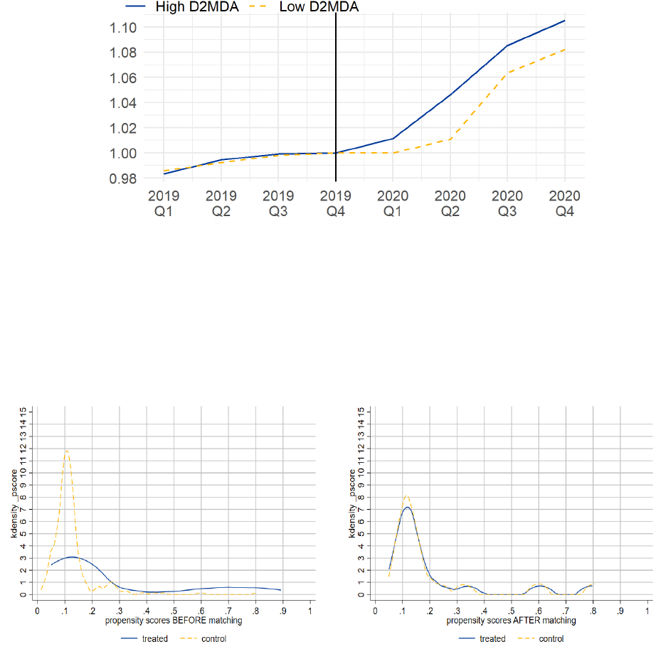
Figure 3. Lending by treated group over 2019Q1-2020Q4
This figure shows the normalised trends of the average bank-firm level logarithmic change in
lending for the group of banks that were in proximity of the MDA trigger (our treatment
group) and the control group over time (2019Q1-2020Q4). Low.D2MDA indicates banks with
an average distance to the MDA in 2019Q2-Q4 below the first quartile of the distance to the
MDA distribution (treated group and blue solid line), whilst High.D2MDA refers to banks with
an average distance to the MDA in 2019Q2-Q4 above the first quartile of the distance to the
MDA distribution (control group and dashed yellow line). Trends are normalised such that both
variables take value 1 in 2019Q4. The black solid vertical line reveals the Covid-19 shock.
Figure 4. Pscore before and after matching (loan-level analysis)
This figure displays Kernel density function of propensity scores between the control (yellow
dashed line) and treatment group (blue solid line) before (left) and after (right) the application
of the propensity score matching approach.
ECB Working Paper Series No 2644 / February 2022
36

Figure 5. Pre-pandemic outstanding share NFCs borrowing by country
This figure displays the average share of total NFC borrowing by country. Share exposed firms
(reported in blue) refers to average share of total NFC borrowing from banks that, prior to the
pandemic (2019Q2-Q4), had an average distance to the MDA trigger below the first quartile
of the distance to the MDA trigger distribution. Share non-exposed firms (reported in yellow)
indicates the average share of total NFC borrowing from banks that, prior to the pandemic
(2019Q2-Q4), had an average distance to the MDA trigger above the first quartile of the distance
to the MDA trigger distribution.
Figure 6. Histogram distance to the MDA
This figure shows the distribution of the average distance to the MDA trigger in 2019Q3-2019Q4.
The y axis displays the percentage while the x axis the lag of the distance to the MDA trigger.
The red dashed vertical line indicates the first quartile of the distance to the MDA trigger
distribution.
ECB Working Paper Series No 2644 / February 2022
37
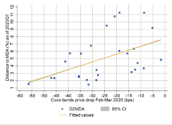
Figure 7. Scatter plot CoCo bond prices and bank distance to MDA trigger point
This figure shows the relationship between the average distance to the MDA trigger in 2019Q2-
Q4 (y-axis) and contingent convertible bonds price drop (x-axix) measured in basis points over
February-March 2020. The price drop is computed as the difference between the highest price
registered in February 2020 against the lowest price registered in March 2020. The blue dots
indicate bank distance to the MDA trigger. The yellow line represents the fitted values coming
from a linear regression model between distance to the MDA trigger and CoCo bond price drop.
The grey shaded area indicates confidence interval at the 95% level.
ECB Working Paper Series No 2644 / February 2022
38

Table 1: Pretreatment bank characteristics
This table shows bank-specific characteristics, averaged for the pretreatment period (2019Q3-Q4), for
the control and the treatment group. The table is divided in two panels. Panel A reports descriptive
statistics for the unmatched sample of bank covariates employed the loan-level analysis (Section 2.1),
whilst Panel B reports desciptive statistics for the matched sample. The PSM applies a logit model and
one-to-three nearest neighbour, imposing a tolerance level on the maximum propensity score distance
(caliper) between the control and the treatment group equals to 0.01. Low.D2MDA indicates banks with
an average distance to the MDA trigger in 2019Q3-Q4 below the first quartile of the distance to the MDA
trigger distribution, whilst High.D2MDA refers to banks with an average distance to the MDA trigger
in 2019Q3-Q4 above the first quartile of the distance to the MDA trigger distribution. Welch t-test
displays the t-statistics coming from the differences between Low.D2MDA and High.D2MDA. L.OCR is
the lag of the Overall Capital Requirement Ratio. L.TA.log is the lag of the logarithm of bank total
assets. L.RW is the lag of risk weight assets-to-total assets ratio. L.MKT FUNDING/TA is the lag
of the debt securities-to-total asset ratio. L.NIM is the lag of the net interest margins. L.NPLs in
the lag of the non-performing loans-to-total loans ratio. L.LIQUID/TA is the lag of the ratio of cash
and financial assets held for trading-to-total assets. L.DIVERS is the lag of the ratio of non-interest
income-to-operating income. L.OFF BS is the lag of the ratio of off-balance sheet activities-to-total
assets. L.LOAN/TA is the lag of the credit exposures-to-total assets ratio. L.CIR is the lag of the cost-
to-income ratio. L.PROVISION/TA is the lag of the ratio of provisions-to-total assets. TLTRO.III is the
ratio of targeted long term refinancing operations III-to-total assets. Sh
Mora is the bank-firm share of
loans under moratorium. Sh Guara is the bank-firm share of loans under government guarantee schemes.
DIVIDEND.REST is the ratio of dividend planned in 2019 but not paid in 2020-to-risk weighted assets.
L.FORBEARANCE is the lag of the ratio of forbearance measures-to-outstanding loans to NFCs. *, **,
*** indicate statistical significance of 1%, 5% and 10% respectively.
High.D2MDA Low.D2MDA Welch test
Panel A: Pre-PSM
L.OCR 0.118 0.113 1.92
∗
L.TA.log 22.96 22.884 0.33
L.RWA/TA 0.49 0.531 -2.35
∗∗
L.MKT FUNDING/TA 0.059 0.068 -0.7
L.NIM 0.015 0.016 -1.72
∗
L.NPL 0.031 0.063 -3.88
∗∗∗
L.LIQUID/TA 0.121 0.121 -0.02
L.DIVERS 0.385 0.388 -0.1
L.OFF BS 0.144 0.168 -1.85
∗
L.LOAN/TA 0.819 0.811 0.58
L.CIR 0.706 0.778 -1.56
L.PROVISION/TA 0.007 0.005 2.52
∗∗
TLTRO.III 0.031 0.043 -1.83
∗
DIVIDEND.REST 0.001 0 0.99
L.FORBEARANCE 0.035 0.036 -0.12
Panel B: Post-PSM
High.D2MDA Low.D2MDA Welch test
L.OCR 0.114 0.113 0.53
L.TA.log 23.367 23.173 0.66
L.RWA/TA 0.503 0.511 -0.36
L.MKT FUNDING/TA 0.088 0.075 0.72
L.NIM 0.016 0.016 0.08
L.NPL 0.055 0.058 -0.3
L.LIQUID/TA 0.114 0.126 -0.65
L.DIVERS 0.369 0.376 -0.26
L.OFF BS 0.179 0.183 -0.18
L.LOAN/TA 0.836 0.818 1.04
L.CIR 0.71 0.713 -0.06
L.PROVISION/TA 0.005 0.005 -0.54
TLTRO.III 0.049 0.046 0.4
DIVIDEND.REST 0.001 0 0.81
L.FORBEARANCE 0.032 0.035 -0.45
ECB Working Paper Series No 2644 / February 2022
39

Table 2: Number of banks by country, by treatment and by matching status
This table reports the number of banks by country, by treatment as well as by matching status.
Low.D2MDA indicates banks with an average distance to the MDA trigger in 2019Q3-Q4 below the first
quartile of the distance to the MDA trigger distribution, whilst High.D2MDA refers to banks with an
average distance to the MDA trigger in 2019Q3-Q4 above the first quartile of the distance to the MDA
trigger distribution. Unmatched sample refers to the pre-PSM sample whilst matched sample indicates
the post-PSM. The PSM applies a logit model and one-to-three nearest neighbour, imposing a tolerance
level on the maximum propensity score distance (caliper) between the control and the treatment group
equals to 0.01.
Control Treated Control Treated
(unmatched) (unmatched) (Matched) (Matched)
AT 45 11 5 6
BE 9 1 3 1
CY 3 2 2 2
DE 85 22 17 18
EE 8 1 2 0
ES 20 8 4 7
FI 9 3 5 3
FR 7 6 3 6
GR 3 4 3 3
IE 10 1 2 1
IT 21 13 18 11
LT 4 1 1 1
LU 13 1 1 1
LV 9 5 1 3
MT 6 2 4 2
NL 13 1 0 1
PT 10 4 4 4
SI 4 5 0 4
SK 3 3 1 2
Total 282 94 76 76
ECB Working Paper Series No 2644 / February 2022
40

Table 3: Summary statistics
This table displays summary descriptive statistics of the variables used
Statistic N Mean St. Dev. Min Pctl(25) Pctl(75) Max
Panel A: Endogenous Variables
∆Log (loans) 3,359,757 0.124 0.626 −1.128 −0.161 0.392 1.985
∆Log (borrowing) 1,038,853 0.335 0.825 −1.232 −0.134 0.739 2.488
∆Log (N.emplo) 1,038,853 −0.008 0.201 −0.693 0.000 0.000 0.624
Panel B: Variables of Interest
Low.D2MDA 5,301,688 0.422 0.494 0.000 0.000 1.000 1.000
L.Dist.MDA 5,301,688 0.062 0.065 0.002 0.026 0.072 0.334
Exp.Firm 5,301,688 0.422 0.494 0.000 0.000 1.000 1.000
Panel C: Control variables
L.OCR 5,301,688 0.105 0.011 0.070 0.097 0.111 0.485
L.TA.log 5,291,458 26.323 1.383 19.424 25.614 27.240 27.240
L.RWA/TA 5,291,458 0.388 0.117 0.156 0.283 0.449 0.811
L.MKT FUNDING/TA 5,291,456 0.147 0.096 0.000 0.090 0.218 0.422
L.NIM 5,259,679 0.013 0.007 0.001 0.010 0.016 0.033
L.NPL 5,277,218 0.045 0.043 0.001 0.023 0.048 0.260
L.LIQUID/TA 5,291,458 0.188 0.134 0.006 0.091 0.248 0.482
L.DIVERS 5,259,679 0.485 0.182 −0.128 0.350 0.605 0.966
L.OFF BS 5,288,863 0.247 0.093 −0.001 0.169 0.336 0.452
L.LOAN/TA 5,291,458 0.786 0.088 0.399 0.758 0.845 0.967
L.CIR 5,253,107 0.696 0.222 0.246 0.601 0.761 2.402
L.PROVISION/TA 5,287,075 0.006 0.004 0.00003 0.004 0.008 0.027
TLTRO.III 5,259,636 0.055 0.049 0.000 0.011 0.095 0.161
S.MORA 4,700,501 0.005 0.062 0.000 0.000 0.000 1.000
S.GUAR 4,700,501 0.157 0.320 0.000 0.000 0.000 1.000
DIVIDEND.REST 5,301,688 0.002 0.003 −0.0005 0.000 0.003 0.024
L.FORBEARANCE 5,244,999 0.028 0.028 0.001 0.009 0.041 0.157
Note: ∆ Log (loans) is the change in bank-firm lending in logarithm. ∆ Log (borrowing) is
the change in the logarithm of a firm’s total borrowing. ∆Log (N.emplo) is the logarithmic
change in the number of employees at the firm level. Low.D2MDA is a dummy variable that
takes the value 1 if a bank has a pre-pandemic distance to the MDA trigger below the first
quartile of the distance to MDA trigger distribution. L.Dist.MDA is the lag of the distance to
the MDA trigger. Exp.Firm is a dummy variable that takes the value 1 for firms that prior to
the pandemic have more than 25% of their credit originating from vulnerable banks. L.OCR is
the lag of the Overall Capital Requirement Ratio. L.TA.log is the lag of the logarithm of bank
total assets. L.RW is the lag of risk weight assets-to-total assets ratio. L.MKT FUNDING/TA
is the lag of the debt securities-to-total asset ratio. L.NIM is the lag of the net interest margins.
L.NPLs in the lag of the non-performing loans-to-total loans ratio. L.LIQUID/TA is the lag of
the ratio of cash and financial assets held for trading-to-total assets. L.DIVERS is the lag of the
ratio of non-interest income-to-operating income. L.OFF BS is the lag of the ratio of off-balance
sheet activities-to-total assets. L.LOAN/TA is the lag of the credit exposures-to-total assets
ratio. L.CIR is the lag of the cost-to-income ratio. L.PROVISION/TA is the lag of the ratio of
provisions-to-total assets. TLTRO.III is the ratio of targeted long term refinancing operations
III-to-total assets. Sh Mora is the bank-firm share of loans under moratorium. Sh Guara is the
ECB Working Paper Series No 2644 / February 2022
41
bank-firm share of loans under government guarantee schemes. DIVIDEND.REST is the ratio
of dividend planned in 2019 but not paid in 2020-to-risk weighted assets. L.FORBEARANCE
is the lag of the ratio of forbearance measures-to-outstanding loans to NFCs.
ECB Working Paper Series No 2644 / February 2022
42

Table 4: Baseline regressions
This table shows the results of the DiD loan-level panel regressions as in equation (1). The quarterly data is collapsed into
pre- and post-event averages. ∆ Log (loans) is the change in bank-firm lending in logarithm. Low.D2MDA is a dummy
variable that takes the value 1 if a bank has a pre-pandemic distance to the MDA trigger below the first quartile of the
distance to MDA trigger distribution. L.OCR is the lag of the Overall Capital Requirement Ratio. L.TA.log is the lag
of the logarithm of bank total assets. L.RW is the lag of risk weight assets-to-total assets ratio. L.MKT FUNDING/TA
is the lag of the debt securities-to-total asset ratio. L.NIM is the lag of the net interest margins. L.NPLs in the lag of
the non-performing loans-to-total loans ratio. L.LIQUID/TA is the lag of the ratio of cash and financial assets held for
trading-to-total assets. L.DIVERS is the lag of the ratio of non-interest income-to-operating income. L.OFF BS is the
lag of the ratio of off-balance sheet activities-to-total assets. L.LOAN/TA is the lag of the credit exposures-to-total assets
ratio. L.CIR is the lag of the cost-to-income ratio. L.PROVISION/TA is the lag of the ratio of provisions-to-total assets.
TLTRO.III is the ratio of targeted long term refinancing operations III-to-total assets. Sh Mora is the bank-firm share of
loans under moratorium. Sh Guara is the bank-firm share of loans under government guarantee schemes. DIVIDEND.REST
is the ratio of dividend planned in 2019 but not paid in 2020-to-risk weighted assets. L.FORBEARANCE is the lag of the
ratio of forbearance measures-to-outstanding loans to NFCs. The PSM matched sample is created via logit model and
one-to-one nearest neighbour, imposing a tolerance level on the maximum propensity score distance (caliper) between the
control and the treatment group equals to 0.01. Standard errors are clustered at bank and firm level. *, **, *** indicate
statistical significance of 1%, 5% and 10% respectively.
Dependent variable: ∆ Log (loans)
Unmatched
Firm FE
Matched
Firm FE
Unmatched
I
˙
LS FE
Matched
I
˙
LS FE
(1) (2) (3) (4)
Low.D2MDA -0.0355
∗∗∗
-0.0926
∗∗∗
-0.0344
∗
-0.0892
∗∗∗
(0.0116) (0.0153) (0.0192) (0.0328)
L.OCR -4.177
∗∗∗
-1.776
∗∗∗
-3.307
∗∗∗
-0.7316
(0.5429) (0.4166) (0.6625) (0.7151)
L.TA.log -0.0048 -0.0091
∗
-0.0159
∗∗
-0.0160
∗∗
(0.0055) (0.0049) (0.0071) (0.0067)
L.RWA/TA -0.0252 -0.1394
∗
-0.0375 -0.1751
(0.0883) (0.0841) (0.1089) (0.1408)
L.MKT FUNDING/TA 0.3844
∗∗∗
0.9188
∗∗∗
0.2268
∗∗
0.6822
∗∗∗
(0.0916) (0.0993) (0.1016) (0.1417)
L.NIM 6.123
∗∗∗
12.32
∗∗∗
6.591
∗∗
8.673
∗∗∗
(1.715) (1.738) (2.600) (2.760)
L.NPL 0.5487
∗∗
0.3989
∗
0.5492 0.8535
∗∗
(0.2312) (0.2182) (0.3686) (0.3551)
L.LIQUID/TA 0.1104 -0.2054 0.2596 -0.3074
(0.0976) (0.1944) (0.1606) (0.2766)
L.DIVERS 0.2353
∗∗∗
0.1514
∗∗
0.2283
∗∗
0.1316
(0.0625) (0.0655) (0.0960) (0.1028)
L.OFF BS -0.0537 0.0270 -0.0345 0.1508
(0.0715) (0.0780) (0.0997) (0.1462)
L.LOAN/TA -0.3495
∗
-0.1298 -0.2605 -0.3650
(0.1820) (0.1452) (0.2757) (0.3117)
L.CIR 0.0199 0.0572 0.0241 0.0364
(0.0254) (0.0474) (0.0405) (0.0618)
L.PROVISION/TA -8.450
∗∗∗
-12.40
∗∗∗
-5.074
∗∗
-12.29
∗∗∗
(1.585) (2.062) (2.040) (3.213)
TLTRO.III -0.1955 -0.4023
∗∗
0.1515 -0.1968
(0.1482) (0.1816) (0.2491) (0.2929)
S.MORA -0.0827
∗∗∗
-0.0860
∗∗∗
-0.0601
∗∗∗
-0.0474
∗∗∗
(0.0127) (0.0180) (0.0135) (0.0159)
S.GUAR 1.463
∗∗∗
1.489
∗∗∗
1.522
∗∗∗
1.570
∗∗∗
(0.0460) (0.0670) (0.0511) (0.0856)
DIVIDEND.REST -0.8782 1.401 -2.050 3.841
(1.791) (3.673) (2.172) (4.458)
L.FORBEARANCE -0.1414 -0.0334 -0.1984 -0.5436
(0.1274) (0.2861) (0.1991) (0.4308)
Fixed-effects
Firm Yes Yes
Bank country Yes Yes Yes Yes
ILS Yes Yes
Fit statistics
Observations 978,055 417,343 2,348,622 1,348,854
R
2
0.70033 0.71066 0.33407 0.31016
Within R
2
0.24896 0.23271 0.21111 0.19100
ECB Working Paper Series No 2644 / February 2022
43

Table 5: Firm-level regressions
This table shows the results of the firm-level panel regressions as in equation (2) and equation (3). The quarterly data
is collapsed into pre- and post-event averages. ∆ Log (borrowing) is the change in firm borrowing in logarithm. ∆Log
(N.employees) is the logarithmic change in the number of employees at the firm level. Exp.Firm. Exp.Firm is a dummy
variable equal to 1 for firms that prior to the pandemic have more than 25% of their credit originating from banks closer
to the MDA trigger point, 0 otherwise. L.OCR is the lag of the Overall Capital Requirement Ratio. L.TA.log is the lag
of the logarithm of bank total assets. L.RW is the lag of risk weight assets-to-total assets ratio. L.MKT FUNDING/TA
is the lag of the debt securities-to-total asset ratio. L.NIM is the lag of the net interest margins. L.NPLs in the lag of
the non-performing loans-to-total loans ratio. L.LIQUID/TA is the lag of the ratio of cash and financial assets held for
trading-to-total assets. L.DIVERS is the lag of the ratio of non-interest income-to-operating income. L.OFF BS is the
lag of the ratio of off-balance sheet activities-to-total assets. L.LOAN/TA is the lag of the credit exposures-to-total assets
ratio. L.CIR is the lag of the cost-to-income ratio. L.PROVISION/TA is the lag of the ratio of provisions-to-total assets.
TLTRO.III is the ratio of targeted long term refinancing operations III-to-total assets. Sh Mora is the bank-firm share of
loans under moratorium. Sh Guara is the bank-firm share of loans under government guarantee schemes. DIVIDEND.REST
is the ratio of dividend planned in 2019 but not paid in 2020-to-risk weighted assets. L.FORBEARANCE is the lag of the
ratio of forbearance measures-to-outstanding loans to NFCs. Standard errors are clustered at firm level. *, **, *** indicate
statistical significance of 1%, 5% and 10% respectively.
∆Log(borrowing) ∆Log(borrowing) ∆log(N.emplo) ∆log(N.emplo)
(1) (2) (3) (4)
Exp.Firm -0.0254
∗∗∗
-0.0301
∗∗∗
-0.0076
∗∗∗
-0.0071
∗∗∗
(0.0030) (0.0034) (0.0011) (0.0013)
Exp.Firm × S.GUAR 0.0297
∗∗∗
-0.0033
(0.0088) (0.0024)
L.OCR -0.3340
∗
-0.3176
∗
0.1348
∗∗
0.1330
∗∗
(0.1851) (0.1852) (0.0608) (0.0615)
L.TA.log -0.0562
∗∗∗
-0.0561
∗∗∗
0.0024
∗∗∗
0.0024
∗∗∗
(0.0017) (0.0017) (0.0004) (0.0005)
L.RWA/TA -0.1692
∗∗∗
-0.1656
∗∗∗
-0.0060 -0.0064
(0.0222) (0.0220) (0.0064) (0.0064)
L.MKT FUNDING/TA 0.9039
∗∗∗
0.9021
∗∗∗
0.0796
∗∗∗
0.0798
∗∗∗
(0.0263) (0.0262) (0.0055) (0.0055)
L.NIM 9.792
∗∗∗
9.782
∗∗∗
0.1460 0.1472
(0.4175) (0.4167) (0.0903) (0.0902)
L.NPL 0.3773
∗∗∗
0.3769
∗∗∗
-0.1125
∗∗∗
-0.1125
∗∗∗
(0.0623) (0.0623) (0.0118) (0.0118)
L.LIQUID/TA 0.2969
∗∗∗
0.3028
∗∗∗
-0.1065
∗∗∗
-0.1071
∗∗∗
(0.0352) (0.0352) (0.0121) (0.0120)
L.DIVERS 0.0843
∗∗∗
0.0875
∗∗∗
0.0432
∗∗∗
0.0428
∗∗∗
(0.0175) (0.0176) (0.0059) (0.0060)
L.OFF BS 0.2031
∗∗∗
0.2051
∗∗∗
-0.0432
∗∗∗
-0.0435
∗∗∗
(0.0296) (0.0296) (0.0045) (0.0045)
L.LOAN/TA -0.5540
∗∗∗
-0.5484
∗∗∗
-0.0730
∗∗∗
-0.0736
∗∗∗
(0.0513) (0.0514) (0.0108) (0.0107)
L.CIR 0.0100 0.0114 -0.0061
∗∗
-0.0063
∗∗
(0.0140) (0.0141) (0.0025) (0.0026)
L.PROVISION/TA -0.0282 -0.0039 -0.2468
∗∗∗
-0.2495
∗∗∗
(0.4762) (0.4751) (0.0876) (0.0873)
TLTRO.III 0.5156
∗∗∗
0.5104
∗∗∗
-0.0426
∗∗∗
-0.0421
∗∗∗
(0.0535) (0.0536) (0.0121) (0.0122)
S.MORA -0.0913
∗∗∗
-0.0908
∗∗∗
-0.0230
∗∗∗
-0.0231
∗∗∗
(0.0083) (0.0083) (0.0039) (0.0039)
S.GUAR 2.050
∗∗∗
2.036
∗∗∗
-0.0065
∗∗∗
-0.0050
∗∗∗
(0.0071) (0.0078) (0.0012) (0.0014)
DIVIDEND.REST -2.287
∗∗∗
-2.377
∗∗∗
-1.048
∗∗∗
-1.038
∗∗∗
(0.4589) (0.4612) (0.1157) (0.1163)
L.FORBEARANCE -1.047
∗∗∗
-1.057
∗∗∗
0.0345
∗∗∗
0.0356
∗∗∗
(0.0597) (0.0598) (0.0130) (0.0133)
Fixed-effects
ILS Yes Yes Yes Yes
Fit statistics
Observations 1,038,844 1,038,844 1,038,844 1,038,844
R
2
0.42228 0.42229 0.10642 0.10642
Within R
2
0.27938 0.27940 0.00189 0.00189
ECB Working Paper Series No 2644 / February 2022
44

Table 6: Placebo test
This table shows the results of the placebo test. The quarterly data is collapsed into pre- and post-event averages. ∆
Log (loans) is the change in bank-firm lending in logarithm. Low.D2MDA is a dummy variable that takes the value 1 if a
bank has a pre-pandemic distance to the MDA trigger below the first quartile of the distance to MDA trigger distribution.
L.OCR is the lag of the Overall Capital Requirement Ratio. L.TA.log is the lag of the logarithm of bank total assets. L.RW
is the lag of risk weight assets-to-total assets ratio. L.MKT FUNDING/TA is the lag of the debt securities-to-total asset
ratio. L.NIM is the lag of the net interest margins. L.NPLs in the lag of the non-performing loans-to-total loans ratio.
L.LIQUID/TA is the lag of the ratio of cash and financial assets held for trading-to-total assets. L.DIVERS is the lag of
the ratio of non-interest income-to-operating income. L.OFF BS is the lag of the ratio of off-balance sheet activities-to-
total assets. L.LOAN/TA is the lag of the credit exposures-to-total assets ratio. L.CIR is the lag of the cost-to-income
ratio. L.PROVISION/TA is the lag of the ratio of provisions-to-total assets. TLTRO.III is the ratio of targeted long
term refinancing operations III-to-total assets. Sh Mora is the bank-firm share of loans under moratorium. Sh Guara is
the bank-firm share of loans under government guarantee schemes. DIVIDEND.REST is the ratio of dividend planned in
2019 but not paid in 2020-to-risk weighted assets. L.FORBEARANCE is the lag of the ratio of forbearance measures-
to-outstanding loans to NFCs. The PSM matched sample is created via logit model and one-to-one nearest neighbour,
imposing a tolerance level on the maximum propensity score distance (caliper) between the control and the treatment
group equals to 0.01. Standard errors are clustered at bank and firm level. *, **, *** indicate statistical significance of 1%,
5% and 10% respectively.
Dependent variable: ∆ Log (loans)
Unmatched
Firm FE
Matched
Firm FE
Unmatched
I
˙
LS FE
Matched
I
˙
LS FE
(1) (2) (3) (4)
Low.D2MDA -0.0048 -0.0218 0.0111 1.33 × 10
−5
(0.0101) (0.0169) (0.0146) (0.0262)
L.OCR -0.0180 -1.043 0.9577 0.1247
(0.4909) (0.7928) (0.6519) (1.015)
L.TA.log -0.0164
∗∗∗
-0.0132 -0.0116
∗
0.0010
(0.0049) (0.0081) (0.0069) (0.0126)
L.RWA/TA -0.2554
∗∗∗
-0.2807
∗∗∗
-0.0908 -0.0080
(0.0799) (0.0801) (0.1095) (0.1246)
L.MKT FUNDING/TA 0.3113
∗∗∗
0.4458
∗∗∗
0.3343
∗∗∗
0.3482
∗∗
(0.0733) (0.1064) (0.1023) (0.1571)
L.NIM 3.352
∗∗∗
4.116
∗∗
3.375
∗
2.414
(1.271) (2.004) (1.802) (2.488)
L.NPL 0.2000 0.0942 -0.2442 -0.5857
(0.1951) (0.3758) (0.3230) (0.5618)
L.LIQUID/TA 0.4996
∗∗∗
0.3726
∗∗∗
0.7479
∗∗∗
0.6478
∗∗∗
(0.0763) (0.0674) (0.0917) (0.1090)
L.DIVERS 0.3509
∗∗∗
0.3387
∗∗∗
0.3648
∗∗∗
0.3684
∗∗∗
(0.0446) (0.0496) (0.0725) (0.0850)
L.OFF BS -0.0847 -0.1346 -0.3373
∗∗∗
-0.4667
∗∗
(0.0814) (0.1251) (0.1202) (0.1800)
L.LOAN/TA 0.7522
∗∗∗
0.3990
∗∗
0.8913
∗∗∗
0.6224
∗∗
(0.1148) (0.1990) (0.1227) (0.3038)
L.CIR -0.0639 -0.0563 -0.0337 -0.0333
(0.0463) (0.0810) (0.0590) (0.1203)
L.PROVISION/TA 0.7747 4.246
∗∗∗
1.794 3.184
(1.816) (1.526) (2.243) (2.715)
L.FORBEARANCE -0.0942 -0.0094 0.1967 0.1175
(0.1630) (0.2077) (0.2181) (0.3154)
Fixed-effects
Firm Yes Yes
Bank country Yes Yes Yes Yes
ILS Yes Yes
Fit statistics
Observations 1,004,489 389,662 2,295,397 1,302,733
R
2
0.64099 0.68361 0.13829 0.13435
Within R
2
0.03637 0.05305 0.04411 0.05890
ECB Working Paper Series No 2644 / February 2022
45

Table 7: Redefinition of the variable of interest: Low.D2MDA
This table shows the results of robustness redefining the Low.D2MDA variable that takes the value 0 only for banks with
a distance to MDA trigger above the last quartile of the distance to the MDA trigger distribution. The quarterly data is
collapsed into pre- and post-event averages. ∆ Log (loans) is the change in bank-firm lending in logarithm. Low.D2MDA is
a dummy variable that takes the value 1 if a bank has a pre-pandemic distance to the MDA trigger below the first quartile
of the distance to MDA trigger distribution. L.OCR is the lag of the Overall Capital Requirement Ratio. L.TA.log is the
lag of the logarithm of bank total assets. L.RW is the lag of risk weight assets-to-total assets ratio. L.MKT FUNDING/TA
is the lag of the debt securities-to-total asset ratio. L.NIM is the lag of the net interest margins. L.NPLs in the lag of
the non-performing loans-to-total loans ratio. L.LIQUID/TA is the lag of the ratio of cash and financial assets held for
trading-to-total assets. L.DIVERS is the lag of the ratio of non-interest income-to-operating income. L.OFF BS is the
lag of the ratio of off-balance sheet activities-to-total assets. L.LOAN/TA is the lag of the credit exposures-to-total assets
ratio. L.CIR is the lag of the cost-to-income ratio. L.PROVISION/TA is the lag of the ratio of provisions-to-total assets.
TLTRO.III is the ratio of targeted long term refinancing operations III-to-total assets. Sh Mora is the bank-firm share of
loans under moratorium. Sh Guara is the bank-firm share of loans under government guarantee schemes. DIVIDEND.REST
is the ratio of dividend planned in 2019 but not paid in 2020-to-risk weighted assets. L.FORBEARANCE is the lag of the
ratio of forbearance measures-to-outstanding loans to NFCs. The PSM matched sample is created via logit model and
one-to-one nearest neighbour, imposing a tolerance level on the maximum propensity score distance (caliper) between the
control and the treatment group equals to 0.01. Standard errors are clustered at bank and firm level. *, **, *** indicate
statistical significance of 1%, 5% and 10% respectively.
Dependent variable: ∆ Log (loans)
Unmatched
Firm FE
Matched
Firm FE
Unmatched
I
˙
LS FE
Matched
I
˙
LS FE
(1) (2) (3) (4)
Low.D2MDA -0.0491
∗∗∗
-0.0752
∗∗∗
-0.0568
∗∗
-0.0425
∗∗
(0.0183) (0.0254) (0.0237) (0.0169)
L.OCR -2.727
∗∗∗
-1.663 -1.255 -1.985
∗∗
(0.8697) (1.349) (1.046) (0.7980)
L.TA.log -0.0006 0.0266
∗∗∗
-0.0034 0.0153
∗
(0.0068) (0.0083) (0.0080) (0.0081)
L.RWA/TA -0.2368
∗∗
-0.1819 -0.1871 -0.4918
∗∗∗
(0.1192) (0.2251) (0.1349) (0.1387)
L.MKT FUNDING/TA 0.8858
∗∗∗
-0.0664 0.6025
∗∗∗
-0.7551
∗∗∗
(0.0942) (0.2408) (0.1285) (0.2286)
L.NIM 9.788
∗∗∗
2.890 5.311
∗
1.236
(2.619) (4.179) (2.913) (2.464)
L.NPL -1.010
∗∗
0.6514
∗
-0.2007 1.496
∗∗∗
(0.4684) (0.3616) (0.5723) (0.3281)
L.LIQUID/TA -0.5041
∗∗
-0.9437
∗∗∗
-0.2919 -1.223
∗∗∗
(0.2155) (0.2943) (0.2212) (0.1997)
L.DIVERS 0.1786
∗
-0.0495 0.1295 -0.2352
∗∗∗
(0.1068) (0.1672) (0.1130) (0.0884)
L.OFF BS -0.2703
∗∗
0.0973 -0.1133 0.2824
(0.1176) (0.1977) (0.1365) (0.1955)
L.LOAN/TA -0.0951 -0.7983
∗∗
0.0468 -1.241
∗∗∗
(0.1984) (0.3145) (0.2481) (0.2332)
L.CIR 0.0997 0.0999
∗∗
0.0651 0.0024
(0.0626) (0.0476) (0.0722) (0.0326)
L.PROVISION/TA -11.74
∗∗∗
-8.511
∗∗
-9.842
∗∗∗
-1.671
(2.380) (3.398) (3.303) (2.283)
TLTRO.III -0.6156
∗∗∗
0.0647 -0.2953 0.1941
(0.2168) (0.2459) (0.2358) (0.2065)
S.MORA -0.0404
∗∗
-0.0449 -0.0333 -0.0449
∗
(0.0187) (0.0343) (0.0202) (0.0235)
S.GUAR 1.453
∗∗∗
1.726
∗∗∗
1.644
∗∗∗
1.896
∗∗∗
(0.0973) (0.0385) (0.0973) (0.0660)
DIVIDEND.REST 14.16
∗∗
39.45
∗∗∗
8.551 15.30
∗
(7.009) (14.11) (7.989) (8.993)
L.FORBEARANCE -0.4306 -0.2049 -1.017
∗∗
0.5321
(0.3492) (0.6329) (0.4466) (0.4224)
Fixed-effects
Firm Yes Yes
Bank country Yes Yes Yes Yes
ILS Yes Yes
Fit statistics
Observations 214,867 64,532 1,052,407 478,172
R
2
0.74402 0.77924 0.36500 0.39334
Within R
2
0.26928 0.31886 0.22421 0.24088
ECB Working Paper Series No 2644 / February 2022
46

Table 8: Continuous specification
This table shows the results of the continuous specification performed on the loan-level panel dataset. The quarterly data
is collapsed into pre- and post-event averages. ∆ Log (loans) is the change in bank-firm lending in logarithm. L.Dist.MDA
is the pre-event average of the distance to the MDA trigger expressed as a continuous variable. L.OCR is the lag of the
Overall Capital Requirement Ratio. L.TA.log is the lag of the logarithm of bank total assets. L.RW is the lag of risk weight
assets-to-total assets ratio. L.MKT FUNDING/TA is the lag of the debt securities-to-total asset ratio. L.NIM is the lag of
the net interest margins. L.NPLs in the lag of the non-performing loans-to-total loans ratio. L.LIQUID/TA is the lag of the
ratio of cash and financial assets held for trading-to-total assets. L.DIVERS is the lag of the ratio of non-interest income-to-
operating income. L.OFF BS is the lag of the ratio of off-balance sheet activities-to-total assets. L.LOAN/TA is the lag of
the credit exposures-to-total assets ratio. L.CIR is the lag of the cost-to-income ratio. L.PROVISION/TA is the lag of the
ratio of provisions-to-total assets. TLTRO.III is the ratio of targeted long term refinancing operations III-to-total assets.
Sh Mora is the bank-firm share of loans under moratorium. Sh Guara is the bank-firm share of loans under government
guarantee schemes. DIVIDEND.REST is the ratio of dividend planned in 2019 but not paid in 2020-to-risk weighted assets.
L.FORBEARANCE is the lag of the ratio of forbearance measures-to-outstanding loans to NFCs. Standard errors are
clustered at bank and firm level. *, **, *** indicate statistical significance of 1%, 5% and 10% respectively.
Dependent variable: ∆ Log (loans)
Unmatched
Firm FE
Unmatched
Firm FE
(1) (2)
L.Dist. MDA 0.5777
∗∗∗
0.2723
(0.1817) (0.2302)
L.OCR -4.166
∗∗∗
-3.374
∗∗∗
(0.5015) (0.6701)
L.TA.log -0.0021 -0.0126
∗
(0.0055) (0.0071)
L.RWA/TA 0.0499 0.0505
(0.0773) (0.0902)
L.MKT FUNDING/TA 0.3701
∗∗∗
0.1907
∗
(0.0865) (0.1110)
L.NIM 5.298
∗∗∗
5.696
∗∗
(1.652) (2.645)
L.NPL 0.5488
∗∗
0.5155
(0.2238) (0.3657)
L.LIQUID/TA 0.1585 0.2708
(0.1215) (0.1879)
L.DIVERS 0.2204
∗∗∗
0.2003
∗
(0.0643) (0.1047)
L.OFF BS -0.0574 -0.0740
(0.0811) (0.1142)
L.LOAN/TA -0.3671
∗
-0.2933
(0.2114) (0.3281)
L.CIR 0.0134 0.0148
(0.0265) (0.0450)
L.PROVISION/TA -7.002
∗∗∗
-3.590
∗
(1.452) (2.041)
TLTRO.III -0.0989 0.2272
(0.1445) (0.2609)
S.MORA -0.0861
∗∗∗
-0.0603
∗∗∗
(0.0124) (0.0137)
S.GUAR 1.459
∗∗∗
1.520
∗∗∗
(0.0462) (0.0512)
DIVIDEND.REST -1.610 -2.403
(1.911) (2.419)
L.FORBEARANCE -0.1456 -0.2059
(0.1273) (0.2050)
Fixed-effects
Firm Yes
Bank country Yes Yes
ILS Yes
Fit statistics
Observations 978,055 2,348,622
R
2
0.70029 0.33392
Within R
2
0.24886 0.21093
ECB Working Paper Series No 2644 / February 2022
47

Table 9: Alternative Matching Approach
This table shows the results of robustness replacing the OCR in the matching strategy with the CET1 ratio. The quarterly
data is collapsed into pre- and post-event averages. ∆ Log (loans) is the change in bank-firm lending in logarithm.
Low.D2MDA is a dummy variable that takes the value 1 if a bank has a pre-pandemic distance to the MDA trigger
below the first quartile of the distance to MDA trigger distribution. L.CET1 is the lag of the common equity tier1 ratio.
L.TA.log is the lag of the logarithm of bank total assets. L.RW is the lag of risk weight assets-to-total assets ratio. L.MKT
FUNDING/TA is the lag of the debt securities-to-total asset ratio. L.NIM is the lag of the net interest margins. L.NPLs in
the lag of the non-performing loans-to-total loans ratio. L.LIQUID/TA is the lag of the ratio of cash and financial assets held
for trading-to-total assets. L.DIVERS is the lag of the ratio of non-interest income-to-operating income. L.OFF BS is the
lag of the ratio of off-balance sheet activities-to-total assets. L.LOAN/TA is the lag of the credit exposures-to-total assets
ratio. L.CIR is the lag of the cost-to-income ratio. L.PROVISION/TA is the lag of the ratio of provisions-to-total assets.
TLTRO.III is the ratio of targeted long term refinancing operations III-to-total assets. Sh Mora is the bank-firm share of
loans under moratorium. Sh Guara is the bank-firm share of loans under government guarantee schemes. DIVIDEND.REST
is the ratio of dividend planned in 2019 but not paid in 2020-to-risk weighted assets. L.FORBEARANCE is the lag of the
ratio of forbearance measures-to-outstanding loans to NFCs. The PSM matched sample is created via logit model and
one-to-one nearest neighbour, imposing a tolerance level on the maximum propensity score distance (caliper) between the
control and the treatment group equals to 0.01. Standard errors are clustered at bank and firm level. *, **, *** indicate
statistical significance of 1%, 5% and 10% respectively.
Dependent variable: ∆ Log (loans)
Unmatched
Firm FE
Matched
Firm FE
Unmatched
I
˙
LS FE
Matched
I
˙
LS FE
(1) (2) (3) (4)
Low.D2MDA -0.0541
∗∗∗
-0.0760
∗∗∗
-0.0536
∗∗
-0.1070
∗∗∗
(0.0164) (0.0183) (0.0248) (0.0297)
L.CET1 -0.2506 -10.10
∗∗∗
-0.4558 -9.871
∗∗∗
(0.2510) (1.948) (0.3358) (1.828)
L.TA.log -0.0045 -0.0365
∗∗
-0.0171
∗∗
-0.0071
(0.0064) (0.0167) (0.0075) (0.0157)
L.RWA/TA -0.0870 -0.9576
∗∗∗
-0.0829 -0.7624
∗∗∗
(0.0949) (0.1940) (0.1151) (0.2101)
L.MKT FUNDING/TA 0.3380
∗∗∗
-0.7189
∗∗∗
0.1932
∗
-1.013
∗∗∗
(0.1043) (0.2650) (0.1134) (0.3023)
L.NIM 6.749
∗∗∗
16.72
∗∗∗
7.144
∗∗∗
10.97
∗∗
(1.850) (4.741) (2.745) (4.337)
L.NPL 0.3836 -1.056
∗
0.4050 -0.3548
(0.2891) (0.5528) (0.4416) (0.5539)
L.LIQUID/TA -0.0853 -0.7473
∗
0.0734 -0.6332
(0.1287) (0.4247) (0.1814) (0.4981)
L.DIVERS 0.2585
∗∗∗
-0.4626
∗∗
0.2437
∗∗
-0.3238
∗
(0.0749) (0.1768) (0.1080) (0.1882)
L.OFF BS 0.1484
∗
0.4496
∗∗
0.1237 0.3000
(0.0812) (0.2217) (0.1112) (0.2529)
L.LOAN/TA -0.4259
∗
-0.5769 -0.3531 -0.0842
(0.2171) (0.6023) (0.2991) (0.6996)
L.CIR 0.0631
∗∗
-0.0893 0.0501 -0.0905
(0.0284) (0.0802) (0.0468) (0.0891)
L.PROVISION/TA -9.418
∗∗∗
-12.09
∗∗∗
-5.790
∗∗
-10.98
∗∗∗
(2.045) (3.058) (2.481) (4.136)
TLTRO.III -0.5944
∗∗∗
0.9168 -0.1583 1.293
∗∗
(0.1642) (0.5856) (0.2446) (0.6343)
S.MORA -0.0830
∗∗∗
-0.0801
∗∗∗
-0.0588
∗∗∗
-0.0139
(0.0142) (0.0298) (0.0125) (0.0096)
S.GUAR 1.465
∗∗∗
1.387
∗∗∗
1.525
∗∗∗
1.473
∗∗∗
(0.0463) (0.0803) (0.0511) (0.0917)
DIVIDEND.REST 1.754 -8.451 -0.5038 -26.62
∗∗
(2.241) (13.80) (2.460) (12.74)
L.FORBEARANCE -0.3865
∗∗
0.4363 -0.4057 0.2647
(0.1641) (0.4078) (0.2474) (0.5269)
Fixed-effects
Firm Yes Yes
Bank country Yes Yes Yes Yes
ILS Yes Yes
Fit statistics
Observations 978,055 100,910 2,348,622 391,809
R
2
0.69950 0.74358 0.33346 0.36103
Within R
2
0.24687 0.27568 0.21039 0.23226
ECB Working Paper Series No 2644 / February 2022
48

Appendix A
Table A. Variables, label, definitions and sources.
Variable Label Definition Source
Dependent variable
Lending ∆ Log (loans) Change in the logarithm of loans from bank i to firm k AnaCredit
Borrowing ∆ Log (borrowing) Change in the logarithm of a firm’s total bank loans AnaCredit
Employment ∆log (N.emplo) Change in the logarithm of a firm’s total number of em-
ployees
Anacredit
Variable of interest
Distance to MDA trigger Low.D2MDA Dummy variable equal to 1 if a bank, in the quarter prior
to the pandemic (2019Q4) has a distance to the MDA
trigger point below the first quartile of the distribution, 0
otherwise
ECB Supervisory
Statistics and au-
thors’ calculations
Exposed firms Exp.Firm Dummy variable equal to 1 for firms that prior to the
pandemic have more than 25% of their credit originating
from banks closer to the MDA trigger point, 0 otherwise
AnaCredit and au-
thors’ calculation
Bank control variables
Overall capital requirements OCR Sum of minimum requirements and the combined buffer
requirements
ECB Supervisory
Statistics
Bank size TA.log Logarithm of bank total assets ECB Supervisory
Statistics and au-
thors’ calculations
Risk weight density RW The ratio of risk-weighted assets-to-total assets ECB Supervisory
Statistics and au-
thors’ calculations
Funding structure MKT FUND-
ING TA
The ratio of debt securities issued-to-total assets ECB Supervisory
Statistics and au-
thors’ calculations
Net interest margin NIM The ratio of interest earning assets minus interest bearing
liabilities-to-total assets ratio
ECB Supervisory
Statistics and au-
thors’ calculations
Non-performing loans NPLs The ratio of non-performing loans-to-gross loans ECB Supervisory
Statistics and au-
thors’ calculations
Liquidity LIQUID/TA The ratio of cash and financial assets held for trading-to-
total assets
ECB Supervisory
Statistics and au-
thors’ calculations
Income stream DIVERS The ratio of non-interest income-to-operating income ECB Supervisory
Statistics and au-
thors’ calculations
Off-balance sheet OFF BS The ratio of off balance sheet activities-to-total assets ECB Supervisory
Statistics and au-
thors’ calculations
Asset composition LOAN/TA The ratio of all credit exposure-to-total assets ECB Supervisory
Statistics and au-
thors’ calculations
Operating efficiency CIR The ratio of operating expenses-to-operating income ECB Supervisory
Statistics and au-
thors’ calculations
Provisions PROVISION/TA The ratio of provisions-to-total assets ECB Supervisory
Statistics and au-
thors’ calculations
Policy control variables
TLTRO III TLTROs III The ratio of targeted longer term refinancing operations-
to-total assets
ECB Market Oper-
ations Database
Moratoria Sh Mora Bank-firm level share of loans from the bank that are sub-
jected to debt moratoria
AnaCredit
Guarantees Sh Guara Bank-firm level share of loans from the bank that are sub-
ject to government guarantees
AnaCredit
Dividend suspension DIVIDEND.REST The ratio of dividend planned in 2019 but not paid in
2020-to-risk weighted assets
Supervisory Data
Forbearance FORBEARANCE The ratio of forbearance take up measure-to-NFC out-
standing loans
Supervisory Data
ECB Working Paper Series No 2644 / February 2022
49

Table B. Correlation Matrix.
(1) (2) (3) (4) (5) (6) (7) (8) (9) (10) (11) (12) (13) (14) (15) (16)
Low.D2MDA 1
L.OCR -0.073 1
L.TA.log -0.018 -0.229 1
TLTRO.III 0.105 -0.155 0.333 1
L.LOAN/TA -0.030 -0.248 0.049 0.162 1
L.CIR 0.092 -0.025 -0.095 -0.007 -0.227 1
L.DIVERS 0.005 0.145 -0.027 -0.056 -0.462 0.058 1
DIVIDEND.REST -0.038 -0.049 0.356 0.076 -0.051 -0.123 -0.002 1
L.FORBEARANCE 0.007 -0.050 -0.104 -0.085 0.024 0.014 0.097 -0.040 1
L.LIQUID/TA 0.001 0.266 0.018 -0.203 -0.871 0.083 0.429 0.109 -0.023 1
L.MKT FUNDING/TA 0.036 -0.078 0.445 0.264 0.106 -0.114 -0.113 0.220 -0.062 -0.050 1
L.NIM 0.088 0.004 -0.254 -0.026 0.151 -0.118 -0.434 -0.107 -0.044 -0.231 -0.305 1
L.NPL 0.260 0.098 -0.143 0.246 -0.175 0.107 0.019 -0.063 0.009 0.046 -0.109 0.321 1
L.OFF BS 0.095 -0.241 0.456 0.213 -0.019 -0.005 0.135 0.175 -0.017 0.090 0.031 -0.123 -0.122 1
L.PROVISION/TA -0.115 -0.226 0.117 -0.028 0.210 0.152 -0.054 -0.055 0.057 -0.269 -0.139 -0.054 -0.145 0.049 1
L.RWA/TA 0.111 -0.048 -0.395 -0.058 0.038 0.038 -0.045 -0.132 0.125 -0.204 -0.369 0.543 0.291 0.053 0.074 1
Note: Low.D2MDA is a dummy variable that takes the value 1 if a bank has a pre-pandemic distance to the MDA trigger below the first
quartile of the distance to MDA trigger distribution. L.OCR is the lag of the Overall Capital Requirement Ratio. L.TA.log is the lag of
the logarithm of bank total assets. L.RW is the lag of risk weight assets-to-total assets ratio. L.MKT FUNDING/TA is the lag of the
debt securities-to-total asset ratio. L.NIM is the lag of the net interest margins. L.NPLs in the lag of the non-performing loans-to-total
loans ratio. L.LIQUID/TA is the lag of the ratio of cash and financial assets held for trading-to-total assets. L.DIVERS is the lag of
the ratio of non-interest income-to-operating income. L.OFF BS is the lag of the ratio of off-balance sheet activities-to-total assets.
L.LOAN/TA is the lag of the credit exposures-to-total assets ratio. L.CIR is the lag of the cost-to-income ratio. L.PROVISION/TA is
the lag of the ratio of provisions-to-total assets. TLTRO.III is the ratio of targeted long term refinancing operations III-to-total assets.
Sh Mora is the bank-firm share of loans under moratorium. Sh Guara is the bank-firm share of loans under government guarantee
schemes. DIVIDEND.REST is the ratio of dividend planned in 2019 but not paid in 2020-to-risk weighted assets. L.FORBEARANCE
is the lag of the ratio of forbearance measures-to-outstanding loans to NFCs.
ECB Working Paper Series No 2644 / February 2022
50

Acknowledgements
The authors are grateful to the Eurosystem Financial Stability Committee Expert Group on banks’ response to the Covid-19 Pandemic
for the constructive discussions. Specifically, we would like to thank Fatima de Silva, Dorian Henricot, Mario Jovanovic, Matías Lamas,
Sandrine Lecapentier, Stefan Schmitz and Leonid Silbermann. We are also indebted to the comments received from colleagues in
Directorate General Macroprudential Policy and Financial Stability of the European Central Bank, among which Sergio Nicoletti Altimari,
Markus Behn, Fatima Pires, Carsten Detken, Jan Hannes Lang, Nikolas Mayer and Cristian Perales. We thank seminar participants at
Bangor University, the Bank of England, Central Bank of Brazil, European Commission, International Monetary Fund, Sveriges
Riksbank, University of Strathclyde and University of Udine. In particular Jose Abad, Awad Rachid, Christoph Bertsch, Gaston Gelos,
Caio Fonseca Ferreira, Petra Lennartsdotter, Jonas Niemeyer and Sole Martinez Peria, Mitra Srobona. All remaining errors are our
responsibility.
Cyril Couaillier
European Central Bank, Frankfurt am Main, Germany; email: Cyril.C[email protected]ropa.eu
Marco Lo Duca
European Central Bank, Frankfurt am Main, Germany; email: marco.lo[email protected]a.eu
Alessio Reghezza
European Central Bank, Frankfurt am Main, Germany; Bangor University, Bangor, United Kingdom;
email: Alessio.Reghez[email protected]pa.eu
Costanza Rodriguez d’Acri
European Central Bank, Frankfurt am Main, Germany; email: Costanza.Rod[email protected]pa.eu
© European Central Bank, 2022
Postal address 60640 Frankfurt am Main, Germany
Telephone +49 69 1344 0
Website www.ecb.europa.eu
All rights reserved. Any reproduction, publication and reprint in the form of a different publication, whether printed or produced
electronically, in whole or in part, is permitted only with the explicit written authorisation of the ECB or the authors.
This paper can be downloaded without charge from www.ecb.europa.eu, from the Social Science Research Network electronic library or
from RePEc: Research Papers in Economics. Information on all of the papers published in the ECB Working Paper Series can be found
on the ECB’s website.
PDF ISBN 978-92-899-4977-4 ISSN 1725-2806 doi:10.2866/08798 QB-AR-22-009-EN-N
