Why do Nigerian Scammers Say They are from Nigeria?
Cormac Herley
Microsoft Research
One Microsoft Way
Redmond, WA, USA
ABSTRACT
False positives cause many promising detection tech-
nologies to be unworkable in practice. Attackers, we
show, face this problem too. In deciding who to attack
true positives are targets successfully attacked, while
false positives are those that are attacked but yield
nothing.
This allows us to view the attacker’s problem as a
binary classification. The most profitable strategy re-
quires accurately distinguishing viable from non-viable
users, and balancing the relative costs of true and false
positives. We show that as victim density decreases the
fraction of viable users than can be profitably attacked
drops dramatically. For example, a 10× reduction in
density can produce a 1000× reduction in the number
of victims found. At very low victim densities the at-
tacker faces a seemingly intractable Catch-22: unless he
can distinguish viable from non-viable users with great
accuracy the attacker cannot find enough victims to be
profitable. However, only by finding large numbers of
victims can he learn how to accurately distinguish the
two.
Finally, this approach suggests an answer to the ques-
tion in the title. Far-fetched tales of West African riches
strike most as comical. Our analysis suggests that is an
advantage to the attacker, not a disadvantage. Since
his attack has a low density of victims the Nigerian
scammer has an over-riding need to reduce false posi-
tives. By sending an email that repels all but the most
gullible the scammer gets the most promising marks to
self-select, and tilts the true to false positive ratio in his
favor.
1. INTRODUCTION: ATTACKERS HAVE
FALSE POSITIVES TOO
False positives have a long history of plaguing secu-
rity systems. They have always been a challenge in
behavioral analysis, and anomaly and intrusion detec-
tion [5]. A force-fed diet of false positives have habit-
uated users to ignore security warnings [15]. In 2010 a
single false positive caused the McAfee anti-virus pro-
gram to send millions of PC’s into never-ending reboot
cycles. The mischief is not limited to computer secu-
rity. Different fields have different names for the inher-
ent trade-offs that classification brings. False alarms
must be balanced against misses in radar [22], precision
against recall in information retrieval, Type I against
Type II errors in medicine and the fraud against the
insult rate in banking [19]. Common to all of these ar-
eas is that one type of error must be traded off against
the other. The relative costs of false positives and false
negatives changes a great deal, so no single solution is
applicable to all domains. Instead, the nature of the
solution chosen depends on the problem specifics. In
decisions on some types of surgery, for example, false
positives (unnecessary surgery) are preferable to false
negatives (necessary surgery not performed) since the
latter can be far worse than the former for the patient.
At the other extreme in deciding guilt in criminal cases
it is often considered that false negatives (guilty per-
son goes free) are more acceptable than false positives
(innocent person sent to jail). In many domains de-
termining to which of two classes something belongs is
extremely hard, and errors of b oth kinds are inevitable.
Attackers, we show, also face this trade-off problem.
Not all targets are viable, i.e., not all yield gain when
attacked. For an attacker, false positives are targets
that are attacked but yield nothing. These must be
balanced against false negatives, which are viable tar-
gets that go un-attacked. When attacking has non-zero
cost, attackers face the same difficult trade-off prob-
lem that has vexed many fields. Attack effort must be
spent carefully and too many misses renders the whole
endeavor unprofitable.
Viewing attacks as binary classification decisions al-
lows us to analyze attacker return in terms of the Re-
ceiver Operator Characteristic (ROC) curve. As an at-
tacker is pushed to the left of the ROC curve social good
is increased: fewer viable users and fewer total users are
attacked. We show that as the density of victims in the
population decreases there is a dramatic deterioration
in the attacker’s return. For example, a 10× reduc-
tion in density can causes a much greater than 1000×
reduction in the number of viable victims found. At
1
very low victim densities the attacker faces a seemingly
intractable Catch-22: unless he can distinguish viable
from non-viable users with great accuracy the attacker
cannot find enough victims to be profitable. However,
only by finding large numbers of victims can he learn
how to accurately distinguish the two. This suggests,
that at low enough victim densities many attacks pose
no economic threat.
Finally, in Section 4, we offer a simple explanation for
the question posed in the title, and suggest how false
positives may be used to intentionally erode attacker
economics.
2. BACKGROUND
2.1 Attacks are seldom free
Malicious software can accomplish many things but
few programs output cash. At the interface between
the digital and physical worlds effort must often be
spent. Odlyzko [3] suggests that this frictional inter-
face between online and off-line worlds explains why
much potential harm goes unrealized. Turning digital
contraband into goods and cash is not always easily
automated. For example, each respondent to a Nige-
rian 419 email requires a large amount of interaction,
as does the Facebook “stuck in London scam.” Cre-
dentials may be stolen by the millions, but emptying
bank accounts requires recruiting and managing mules
[7]. The endgame of many attacks require per-target
effort. Thus when cost is non-zero each potential target
represents an investment decision to an attacker. He
invests effort in the hopes of payoff, but this decision is
never flawless.
2.2 Victim distribution model
We consider a population of N users, which contains
M viable targets. By viable we mean that these tar-
gets always yield a net profit of G when attacked, while
non-viable targets yield nothing. Each attack costs C;
thus attacking a non-viable target generates a loss of
C. We call d = M/N the density of viable users in the
population.
We assume that some users are far more likely to be
viable than others. Viability is not directly observable:
the attacker doesn’t know with certainty that he will
succeed unless he tries the attack. Nonetheless, the
fact that some users are better prospects than others
is observable. We assume that the attacker has a sim-
ple score, x, that he assigns to each user. The larger
the score, the more likely in the attacker’s estimate the
user is to be viable.
More formally, the score, x, is a sufficient statistic
[22]. The attacker might have several observations about
the user, where he lives, his place of work, the accounts
he possesses, etc: all of these be reduced to the single
numeric quantity x. This encapsulates all of the observ-
able information about the viability of User(i). Without
loss of generality we’ll assume that viable users tend
to have higher x values than non-viable ones. This
does not mean that all viable users have higher val-
ues that non-viable ones. For example, we might have
pdf(x | non-viable) = N (0, 1) and pdf(x | viable) =
N (µ, 1). Thus, the observable x is normally distributed
with unit variance, but the mean, µ, of x over viable
users is higher than over non-viable users. An example
is shown in Figure 2.
The viability depends on the specific attack. For ex-
ample, those who live in wealthier areas may be judged
more likely to be viable under most attacks. Those who
are C-level officers at large corporations might be more
viable of elaborate industrial espionage or Advanced
Persistent Threat attacks, etc. Those who have fallen
for a Nigerian scam, may be more likely to fall for the
related “fraud funds recovery” scam.
It is worth emphasizing that rich does not mean vi-
able. There is little secret about who the richest people
in the world are, but attacking the Forbes 100 list is not
a sure path to wealth. To be viable the attacker must
be able to successfully extract the money (or other re-
source he targets). For example, if an attacker gets key-
logging malware on a user’s machine, harvests banking
passwords but cannot irreversibly transfer money from
the account this counts as a failure not a success. This
is a cost to the attacker for no gain.
2.3 Attack model
For now we assume a single attacker. He decides
whether to attack User(i) based on everything he knows
about how likely User(i) is to be viable, i.e., based on
his observation of x
i
. His expected return from attack-
ing a user with observable x
i
is:
P {viable | x
i
} · G − P {non-viable | x
i
} · C.
Clearly, the best case for the attacker is to attack if
P {viable | x
i
} · G > P {non-viable | x
i
} · C. He can
never do better, but can easily do worse. The attacker
does not of course know P {viable | x
i
}; he generally es-
timates it from his previous experience. The particular
problem that this poses when victim density is low is
explored in Section 3.7.
In an attack campaign the true positive rate, t
p
, is the
fraction of viable targets attacked, and the false positive
rate, f
p
is the fraction of non-viable targets attacked.
That is, t
p
is the number of viable users attacked di-
vided by the total number of viable users. Similarly,
f
p
is the number of non-viable users attacked divided
by the total number of non-viable users. Thus the at-
tacker will attack d·t
p
·N viable users and (1−d)·f
p
·N
non-viable users. The expected return is then:
E{R} = (d · t
p
· G − (1 − d) · f
p
· C) · N. (1)
2

Our attacker risks two types of errors. Sometimes he
will attack a non-viable user and gain nothing (thereby
losing C), sometimes he will decide not to attack a vi-
able user (thereby foregoing a net gain of G). Thus
he faces a binary classification problem. Every attack
results in either a true positive (viable user found) or
false positive (non-viable user found). Ideal classifica-
tion requires that the attacker know exactly which users
will repay effort and which will not, and never makes
the mistake of attacking unnecessarily or of leaving a
viable target alone.
2.4 ROC curves
The trade-off between the two types of error is usually
graphed as a Receiver Operator Characteristic (ROC)
curve (i.e., t
p
vs. f
p
) [22], an example of which is shown
in Figure 1. The curve represents the ability to discrim-
inate between viable and non-viable targets. Any point
on the ROC curve represents a possible operating point
or strategy for the attacker.
For example, one strategy is for the attacker to choose
a threshold x
∗
and attack User(i) if x
i
> x
∗
. The ROC
curve is then generated by plotting the true and false
positive rates achieved as we sweep x
∗
through all pos-
sible values. The actual shape of the ROC curve is
determined solely by the distribution of x over viable
and non-viable users. In fact, the ROC curve is the
graph of cdf(x | viable) vs. cdf(x | non-viable).
Three easily-proved properties of ROC curves [22] will
be useful in the following.
• The ROC curve is monotonically increasing: the
true positive rate t
p
is an increasing function of
the false positive rate f
p
.
• The ROC curve has monotonically decreasing slope:
the slope dt
p
/df
p
is a decreasing function of f
p
.
• The Area Under the Curve (AUC) is the proba-
bility that the classifier ranks a randomly chosen
true positive higher than a randomly chosen false
positive.
The first property, monotonicity, presents our attacker
with his fundamental tradeoff. Since he is constrained
to move on the ROC curve, the attacker can decrease
false positives only by decreasing true positives and vice
versa. Thus, his attack strategy must weigh the number
of both types of error and their relative costs [22].
The AUC is often taken as a figure of merit for a
classifier. The AUC for the ROC curve shown in Figure
1 is 0.9. This means that for a randomly chosen viable
user i and a randomly chosen non-viable user j we will
have x
i
> x
j
90% of the time. Clearly, the higher AUC
the better the classifier.
2.5 Attack everyone, attack at random
Figure 1: Example ROC curve showing the
tradeoff between true and false positives. The
point with unit slope tangent is profitable only
if attacking everyone is profitable. Otherwise
profitable strategies lie only to the left of that
point.
The diagonal line in Figure 1 represents a random
classifier, which makes decisions that are no better (and
no worse) than random. That is, targets are attacked
with uniform probability 1/N . Any curve above this
line is a better-than-random classifier: for a given false
positive rate it achieves more true positives than the
random classifier.
When attacking everyone t
p
= 1 and f
p
= 1. That
is all viable and non-viable targets are attacked. When
this happens the expected return is: E{R} = (d · G −
(1−d)·C)·N. Imposing the constraint that the expected
return should be positive, E{R} > 0, gives:
d =
M
N
>
C
G + C
. (2)
If this holds, then attacking everyone is a profitable
proposition.
When C > 0 there is an intuitive explanation for this
constraint. Attacking everyone is profitable so long as
the density of viable targets is greater than the ratio
of the costs of unsuccessful and successful attacks. For
example, if 1% of users are viable targets then the net
gain from a successful attack would have to be 99× the
cost of an attack to make targeting the whole popula-
tion profitable.
Attacking at random (i.e., ignoring the score x
i
) has
the same expected return as attacking everyone.
In the special case where C = 0 (i.e., it costs nothing
to attack) making a profit is easy so long as there are
3

some viable victims. Profit is guaranteed so long as true
positives give some gain. Spam seems to be an exam-
ple where C ≈ 0. If false positives cost nothing, while
false negatives mean lost income, there’s little point in
restraint. Equally, if G → ∞ this strategy makes sense:
if an attacker has infinite resources and places infinite
value on each viable target he will attack everyone. In
this paper we will assume that C > 0 and G is finite.
2.6 Optimal Operating Point
Since the slope of the ROC curve is decreasing the
best ratio of true to false positives is in the lower left cor-
ner. In this region true positives are increasing rapidly,
while false positives are increasing slowly. Going fur-
ther right on the ROC involves adding false positives at
an increasing rate. Operating in the lower left corner
essentially involves attacking only targets that are al-
most “sure things.” The problem with this strategy is
that by going after only “sure things” it leaves most of
the viable targets un-attacked.
For a single attacker the return is given by (1). This
is maximized when dE{R}/df
p
= 0, which gives:
dt
p
df
p
=
1 − d
d
·
C
G
. (3)
Thus, to maximize return, the attacker should operate
at the point on the ROC curve with this slope. We refer
to this point as the Optimal Operating Point (OOP).
The point can be found by drawing a tangent with this
slope to the ROC curve. Note that the slop e at the
OOP is determined by the density of viable targets in
the population, and the ratio of net gain to cost.
Operating at this point does not mean that no vi-
able victims will be found at operating points further
to the right. However, if he moves to the right of the
OOP, our attacker finds that the cost of false positives
that are added now more than consumes the gain from
true positives that are added. Optimality requires that
many viable targets to the right are ignored. For max-
imum profit, the attacker does not attempt to find all
viable targets, he tries to find the most easily found
ones. Pursuing the least-likely viable targets (i.e., those
with smallest x values) makes no sense if they cannot
be easily distinguished from false positives.
Operating to the right of the OOP makes no sense,
however there are several good reasons why an attacker
might operate to the left. To meet a finite budget, or
reduce the variance of return an attacker might operate
far to the left of the OOP. We explore these reasons in
Section 3.6. Thus the return achieved at the OOP can
be considered an upper bound (and sometimes a very
loose one) on what can be achieved.
3. ROC CURVES AND THE PURSUIT OF
PROFIT
Quantity Symbol
Number of users N
Number of viable users M
Victim density d = M/N
Net gain from viable user G
Cost of attack C
True positive rate t
p
False positive rate f
p
Number viable users attacked d · t
p
· N
Number non-viable users attacked (1 − d) · f
p
· N
Table 1: Summary of notation and symbols used
in this paper.
Having reviewed the basics of ROC curves we now
explore some implications for our attacker. The best
that an attacker can do is to op erate at the point with
slope given in (3). We assume that our attacker finds
this point, either by analysis or (more likely) trial and
error. We now explore the implications of the trade-
off between true and false positives for the attacker’s
return.
3.1 As slope increases fewer users are attacked
We now show that as the slope at the OOP increases
fewer users are attacked. Recall, from Section 2.4, that
the ROC curve is monotonically increasing, but that
its slope is monotonically decreasing with f
p
. It follows
that increasing slope implies decreasing f
p
which in turn
implies decreasing t
p
. Thus, the higher the slope at the
OOP, the lower both the true and false positive rates t
p
and f
p
.
This is significant because as our attacker decreases t
p
and f
p
he attacks fewer viable users (i.e., d · t
p
· N is de-
creasing) and fewer total users (i.e., d·t
p
·N +(1−d)·f
p
·
N is decreasing). Thus, as slope increases not only are
fewer total targets attacked, but fewer viable targets are
attacked. Thus the global social good is increased as the
attacker retreats leftwards along the ROC curve. This
is true whether our goal is to reduce the total number
of targets attacked or the total number of viable targets
attacked.
Pictorially this can be seen in Figure 1. At the top-
right of the ROC curve, everyone is attacked and all
viable targets are found. Here t
p
= 1 and f
p
= 1.
This appears to be the case of broadcast attacks such
as spam. These attacks are bad, not merely because vi-
able victims are found and exploited, but all users suffer
the attacks. It can reasonably be argued for broadcast
attacks that the harm to the non-viable population is
many times greater than the value extracted from the
viable population. At the other extreme, in the bottom-
left of the ROC curve nobody is attacked and no viable
targets are found (i.e., t
p
= 0 and f
p
= 0). Clearly,
pushing the attacker to the left on his ROC curve is
4

Figure 2: Distribution of x for normally dis-
tributed scores. The mean over non-viable users
is zero (left-most curve). Various assumptions
of the separation between viable and non-viable
users are given. Means of µ = 1.18, 2.32 and 3.28
result in the classifiers of Figure 3 which have
90%, 95% and 99% ability to tell randomly cho-
sen viable users from non-viable.
very desirable.
3.2 If attacking everyone is not profitable slope
must be greater than unity
We now show that the OOP must have slope > 1
unless attacking everyone is profitable. Suppose that
the slope at the OOP is less than unity. From (3) this
implies:
1 − d
d
·
C
G
< 1.
Rearranging gives:
d >
C
G + C
which is the same as (2), the condition to guarantee
that attacking everyone is profitable. Thus, if attacking
everyone is not profitable, then the slope at the OOP
must be greater than unity.
Hence (when attacking everyone is not profitable) a
line tangent to the ROC curve with unity slope estab-
lishes the point that is an upper bound on the true and
false positive rates achievable with a given classifier.
For example, in Figure 1 the tangent with unity slope
intersects the ROC curve at (f
p
, t
p
) ≈ (0.182, 0.818).
Thus 81.8% is an upper bound on the fraction of viable
targets that will be attacked using the optimal strategy.
Similarly, 18.2% is an upper bound on the fraction of
non-viable targets that will b e attacked.
Since we assume merely that attacking all users is not
profitable both of these bounds are very loose. They
are instructive nonetheless. The absolute best of cir-
cumstances, for this ROC curve, result in a little over
80% of viable targets being attacked. An attacker who
does not face comp etition from other attackers, who
Figure 3: ROC curves for a single attacker with
perfect knowledge. The observables are nor-
mally distributed for both viable and non-viable
users with only the mean changing. The AUC
(i.e., probability that the attacker can tell a vi-
able user from non-viable) are 90%, 95% and
99%.
has perfect information about the viability probabili-
ties, and who knows precisely the density, d, of viable
victims in the population will still attack no more than
81.8% of viable targets when maximizing his profit in
this example. If we relax any of these assumptions then
he maximizes his profit by attacking even fewer viable
targets. We examine deviations from the ideal case in
Section 3.6.
The argument at unity slope can be (approximately)
repeated at other (higher) slopes. If attacking all of the
top 1/W is profitable then attacking a population with
density dW is profitable in which case (2) gives
d >
C
W · ( G + C)
.
From (3) if the slope at the OOP is less than W then
d >
C
W · G + C
.
The second constraint is looser than the first, but only
by a little if we assume that G ≫ C (i.e., gain from
successful attack is much greater than cost). Thus, if
attacking the top 1/W of the population (sorted in de-
scending order of viability estimate x
i
) is not profitable
then the slope at the OOP ≈ W. For expensive attacks,
the slope at the OOP will be very high. For example,
where attacking all of the top 1% of the population is
not profitable, the slope must be about 100. In the ex-
5
ample ROC curve shown in Figure 1 this is achieved at
t
p
= 0.0518 and f
p
= 0.00029; i.e., only 5.18% of viable
victims are attacked. If attacking all of the top 0.1% of
the population is not profitable then we might expect a
slope of about 1,000, which is achieved at t
p
= 0.0019
so that only 0.19% of viable victims would be attacked.
This pushes the attacker to the extreme left of the ROC
curve, where (as we saw in Section 3.1) social good is
increased and fewer users are attacked.
3.3 As density decreases slope increases
Observe that as the density of viable targets, d, de-
creases, the slope at the OOP (given in (3)) increases.
Recall (from Section 2.6) that the slope of the ROC
curve is monotonically decreasing. Thus, as d → 0,
the optimal operating point will retreat leftward along
the ROC curve. As we’ve seen in Section 3.1 this means
fewer true positives and fewer total users attacked. Hence,
as the number of viable targets decreases the attacker
must make more conservative attack decisions. This is
true, even though the gain G, cost C and ability to dis-
tinguish viable from non-viable targets is unchanged.
For example, suppose, using the ROC curve of Figure
1, an attack has G/C = 9, i.e., the gain from a success-
ful attack is 9× the cost of an unsuccessful one. Further
suppose d = 1/10 which makes the slope at the OOP
equal to one. We already saw that the unity slope tan-
gent resulted in only 81.8% of viable targets and 18.2%
of non-viable targets being attacked. Since d = 1/10
we have that 10% of users are viable targets. Thus,
0.818×0.1 = 0.0818 or 8.18% of the population are suc-
cessfully attacked and 0.818 × 0.1 + 0.182 × 0.9 = 0.246
or 24.6% of all users will be attacked.
Now suppose that the density is reduced by a factor
of 10 so that d = 1/100. Everything else remains un-
changed. From (3) the slope at the OOP must now be:
100 × (1 − 1/100) × 1/9 = 11. Not shown, but the tan-
gent with this slope intersects the ROC curve in Figure
1 at approximately t
p
= 0.34 and f
p
= 0.013. Thus, the
optimal strategy now attacks only 34.0% of viable tar-
gets and 1.3% of non-viable targets. Since d = 1/100
we have that 1% of users are viable targets. Thus,
0.34×0.01 = 0.0034 or 0.34% of the population are suc-
cessfully attacked and 0.34×0.01+0.013×0.99 = 0.0163
or 1.63% of all users are attacked. Hence, in this case, a
10× reduction in the victim density reduces the number
of true positives by almost 24× and the number of all
attacked users by about 15 × .
While the exact improvement depends on the particu-
lar ROC curve, dramatic deterioration in the attacker’s
situation is guaranteed when density gets low enough.
Independent of the ROC curve, it is easy to see from
(3) that a factor of K reduction in density implies at
least a factor of K increase in slope (for K > 1). For
many classifiers the slope of the ROC tends to ∞ as
f
p
→ 0. (We show some such distributions in Section
3.4.) Very high slope for small values of density implies
that the true positive rate falls very quickly with further
decreases in d.
3.4 Different ROC Curves
We have used the ROC curve of Figure 1 to illustrate
several of the points made. While, as shown in Section
3.3, it is always true that decreasing density reduces the
optimal number of viable victims attacked the numbers
given were particular to the ROC curve, gain ratio G/C
and density d chosen. We now examine some alterna-
tives.
As stated earlier, a convenient parametric model is to
assume that pdf (x | viable) and pdf(x | non-viable)
are drawn from the same distribution with different
means. For example, with unit-variance normal dis-
tribution we would have pdf(x | non-viable) = N (0, 1)
and pdf(x | viable) = N (µ, 1). That is, by choosing µ we
can achieve any desired degree of overlap between the
two populations. This is shown in Figure 2 for three dif-
ferent values of µ. When µ is small the overlap between
N (0, 1) and N (µ, 1) is large and the classifier cannot
be very good. As µ increases the overlap decreases and
the classifier gets better.
The ROC curves for the distributions shown in Figure
2 are given in Figure 3 with values of AUC= 0.9, 0.95
and 0.99. The rightmost curve in Figure 2 corresponds
to the uppermost (i.e., best) classifier in Figure 3. These
correspond to an attacker ability to distinguish ran-
domly chosen viable from non-viable 90%, 95% and 99%
of the time. The highest curve (i.e., AUC = 0.99) is
clearly the best among the classifiers.
This parametric model, using normal distributions is
very common in detection and classification work [22].
It has an additional advantage in our case. Viability
often requires the AND of many things; for example
it might require that the victim have money, and have
a particular software vulnerability, and do banking on
the affected machine and that money can be moved ir-
reversibly from his account. The lognormal distribution
is often used to model variables that are the product of
several positive variables, and thus is an ideal choice
for modeling the viability variable x. Since the ROC
curve is unaffected by a monotonic transformation of
x the curves for pdf(x | non-viable) = ln N (0, 1) and
pdf(x | viable) = ln N ( µ, 1) are identical to those plot-
ted in Figure 3.
In Figure 4 we plot the slope of each of these ROC
curves as a function of log
10
t
p
. These show that large
slopes are achieved only at very small true positive
rates. For example, a slope of 100 is achieved at a true
positive rate of 5.18%, 20.6% and 59.4% by the curves
with AUC of 0.9, 0.95 and 0.99 respectively. Similarly, a
slope of 1000 is achieved at 0.19%, 3.52% and 32.1% re-
6

Figure 4: Slope versus true positive rate, t
p
, for
the curves shown in Figure 3. Observe that
when the slope must be high, the true posi-
tive rate falls rapidly. Even for the best clas-
sifier (upper curve) a slope of 1000 is achieved
at t
p
= 0.321 ≈ log
10
(−0.494).
spectively. Thus, for example, if the density d and gain
ratio G/C indicated that the OOP should have slope
1000 then an attacker using the AUC= 0.95 classifier
would optimally attack only 3.52% of viable users.
If we fix G/C we can plot the true positive rate, t
p
,
as a function of victim density, d. This has been done
in Figure 5 (a) using a value of G/C = 20 and (b) us-
ing a value of G/C = 100. For example, from Figure
5 (a), using the AUC= 0.95 classifier the true p ositive
rate will be 0.683, 0.301, 0.065 and 0.0061 when victims
represent 1%, 0.1%, 0.01% and 0.001% of the popula-
tion respectively. To emphasize: low victim densities
results in smaller and smaller fractions of the viable
victims being attacked.
Finally, in Figure 6 (a) and (b) we plot the fraction
of the population successfully attacked (i.e., d · t
p
vs.
d) again using values of G/C = 20 and 100. Observe
that the fraction of the population attacked always falls
faster (and generally much faster) than d. For example,
when G/C = 100 and AUC=0.9 a factor of 10 reduction
of d from 10
−5
to 10
−6
causes about a factor of 1000
reduction in the fraction of the population successfully
attacked.
3.5 Diversity is more important than strength
The dramatic fall of the fraction victimized with d
shown in Figure 6 suggests that many small attack op-
portunities are harder to profitably exploit than one big
one. We now show that this is indeed the case. From
the attacker’s point of view the sum of the parts is a lot
smaller than the whole.
Recall, for an attack campaign, that the numb er of
victims found is d · t
p
· N. Suppose we have two tar-
get populations each with viable victim densities d/2.
Let’s compare the two opportunities with densities d/2
with a single opportunity with density d. Assume that
the distribution of scores x doesn’t change. Thus, all
three will have the same shaped ROC curve (since the
ROC curve depends only on the distribution of the x
i
),
though different OOP’s will be appropriate in exploit-
ing them (since the OOP depends on d). For clarity, in
the remainder of this section we will label t
p
and f
p
as
being explicit functions of density; e.g., t
p
(d/2) is the
true positive rate for the opportunity with density d/2
etc.
Since t
p
is monotonically decreasing with slope, and
slope at the OOP is monotonically increasing as d de-
creases we have t
p
(d/2) < t
p
(d). Thus,
d/2 · t
p
(d/2) · N + d/2 · t
p
(d/2) · N < d · t
p
(d) · N.
The left-hand side is the number of viable victims at-
tacked in the two opportunities and the right-hand side
is the numb er attacked in the single joint opportunity.
Thus, the attacker gets fewer victims when attacking
two small populations than when attacking a larger
population.
For example, consider the ROC curve shown in Fig-
ure 1. Suppose there are d · N = (d/2 + d/2) · N targets
in the overall population. Suppose the optimal oper-
ating point (given by (3)) dictates a slope of 11 when
attacking the opportunity with density d. We already
saw that this corresponds to a value of t
p
(d) = 0.340
in Figure 1. Thus, d · 0.340 × N users become vic-
tims. Now, if we split the viable victims into two pop-
ulations of density d/2 the slope at the OOP must be
> 22. This occurs at t
p
(d/2) = 0.213 in Figure 1. Thus,
d/2 · 0.213 · N + d/2 · 0.213 · N = d · 0.213 · N users
become victims; i.e., the true positive rate (the fraction
of viable users attacked) has fallen from 34% to 21.3%.
This benefit of diversity becomes even more obvious
as we continue to split the target pool into small groups.
Suppose the targets are divided into 20 categories, each
representing a viable density of d/20. The OOP must
now have slope > 20 × 11 = 220. The point with slope
220 in Figure 1 occurs at t
p
= 0.01962. Thus, over these
20 opportunities 1.96% of users b ecome victims, a fac-
tor of 17× lower than if they were part of the same vul-
nerability pool. Thus, when presented with 20 smaller
vulnerable populations the attacker successfully attacks
a factor of 17× fewer users. Diversity in the attacks that
succeed hugely improves the outcome for the user pop-
ulation, even when there is no change in the number of
vulnerable users or the cost and gain associated with
attacks.
3.5.1 Everybody vulnerable, almost nobody attacked
7

The number of viable users attacked for a single at-
tack of density d is d · t
p
(d) · N. If we divide into Q
different opportunities of size d/Q the number of viable
victims attacked is:
d
Q
·
Q
∑
k=1
t
p
(d/Q) · N = d · t
p
(d/Q) · N.
Since t
p
(d/Q) ≪ t
p
(d) for large Q the fragmented op-
portunity is always worse for the attacker than the sin-
gle large opportunity.
In fact, as shown in Figure 4, t
p
(d/Q) can be made
arbitrarily small for large Q. Thus it is trivially easy to
construct scenarios where 100% of the population is vi-
able, but where the most profitable strategy will involve
attacking an arbitrarily small fraction. For example, if
we choose d = 1 (everyone viable) and Q large enough
so that t
p
(d/Q) < 0.01 then all users are viable, but the
optimal strategy attacks fewer than 1% of them. Con-
sulting Figure 5 (a), for example, we see that for the
AUC= 0.9 classifier the true p ositive rate at d = 10
−4
is < 0.01. Thus, if we have 10,000 distinct attack types,
each of which has a density of 1-in-10,000 then the en-
tire population is vulnerable and viable, and yet the
optimal strategy for the attacker results in fewer than
1% of users being victimized.
This helps formalize the observation that diversity is
important in avoiding attacks [11] and explains why at-
tacks appropriate to small victim densities are of little
concern to the whole p opulation.
3.6 Deviations from the Ideal
3.6.1 Budget-constrained attacker
We chose G/C = 20 and G/C = 100 in Figure 5 to
illustrate the decay of profitability with density: as the
density of viable victims decreases the fraction of that
decreasing population that can be successfully iden-
tified shrinks. Even with good classifiers it appears
that attacks with very small victim densities are hard
to attack profitably. For example, when G/C = 100
and AUC= 0.9 if 1-in-100,000 users are viable, then
t
p
= 0.04. That is, a population of 200 million users
will contain 2000 viable users, of which 80 will be at-
tacked using the optimal strategy. Fully, 96% of the
viable users (who succumb if attacked and yield a 100×
payback for the investment) will escape harm because
there is no strategy to attack them without also attack-
ing so many non-viable users as to destroy the profit.
The example numbers we have chosen G/C = 20 and
G/C = 100 might appear small. That is, might it not
be possible that the gain, G, is not 20 or 100 times
the cost of an attack, but 1000 or 10,000 or a million?
Low success rates happen only when the slope at the
OOP is high. Very high values of G/C would have (3)
imply modest values of slope at the OOP even at small
densities. We argue now against this view. In fact, if
G/C is very large the attacker may have to be even
more conservative.
The rate of change of t
p
with resp ect to f
p
at the
OOP is given by (3). At this point the attacker finds
one viable user for every
d
1 − d
·
dt
p
df
p
=
G
C
false positives. Effectively, his return resembles a G/C+
1 sided coin. He gains G when the desired side comes
up, but otherwise loses C. The strategy is optimal and
profitable on the average: if he plays long enough he
wins the maximum possible amount. However, the vari-
ance of the return is very high when the number of at-
tacks on the order of O(G/C). For example, suppose
G/C = 1000 and d = 10
−4
. The probability of not find-
ing a single victim after 1000 attacks is binocdf(0, 1000, 0.001)
= 36.8%. If this happens the attacker is severely in the
red. To be concrete, if C = $20 he is down $20,000,
and even a successful attack won’t put him back in the
black. The fact that operating at the OOP is the most
profitable strategy is of little consolation if he has a fixed
budget and doesn’t find a victim before it is exhausted.
For example, at $20 per attack, an attacker who starts
with a fixed budget of $10,000 would find it exhausted
with probability binocdf(0, 500, 0.001) = 60.1% before
he found his first victim. Echoing Keynes we might
say that the victims can stay hidden longer than our
attacker can stay solvent.
Thus, a budget-constrained attacker, at least in the
beginning, must be very conservative. If he needs a
victim every 20 attacks then he must operate at a point
with slope
1 − d
d
·
1
20
rather than
1 − d
d
·
C
G
.
Hence, even if G/C is very large, he cannot afford the
risk of a long dry patch before finding a profitable vic-
tim. This hugely influences the conservatism of his
strategy. For example, if d = 10
−4
and G/C = 1000,
the optimal strategy would have the attacker operate at
the point on the ROC with slope ≈ 10 but if ne needs
a victim every 20 attacks he would operate at a point
with slope 500. Figure 4 shows the dramatic effect this
has on the true positive rate.
Similarly, when G/C is large the variance of the re-
turn is very high at the OOP. The attacker finds one
victim on average in every G/C+1 attempts. The mean
number of victims found after k attacks is k · C/G, but
the variance is (1 − C/G) · k · C/G. Thus, returns will
vary wildly. As before, if he has resources and can play
long enough, it evens out. However, to persevere in a
strategy that has a 36.8% chance of delivering zero vic-
tims after k = G/C = 1000 attacks requires confidence
that our attacker has not mis-estimated the parameters.
8

In Section 3.6.2 we show that optimistic assessments of
victim density, classifier accuracy or gain ratio can re-
duce the return by orders of magnitude. However, the
attacker has no real way of estimating any of these pa-
rameters except by trial and error. Thus an attacker
who goes 500 attacks without a victim has no good way
of determining whether this the expected consequences
of operating at the OOP when G/C is high (and prof-
itable victims will come with persistence) or whether he
has entirely overestimated the opportunity (and his at-
tack strategy will bankrupt him if he perseveres). While
victim density, classifier accuracy and gain ratio might
remain relatively stable over time if a single attacker has
the opportunity to himself, this might not be the case if
other attackers b egin to target the same viable victim
pool. For all of these reasons we argue that, even when
G/C is high, the attacker will not operate at the OOP
with slope given by (3) but at a far more conservative
point with slope:
1 − d
d
·
1
k
max
, (4)
where k
max
is the maximum average number of attacks
he is willing to go between successes. This value, k
max
,
is determined by his fear of exhausting his budget, hav-
ing too high a variance and having density decrease due
to factors such as other attackers joining the pool.
3.6.2 Optimism does not pay
The analysis for optimum profit assumes several things.
It assumes that the attacker knows the density of viable
victims d, the gain ratio G/C and correctly chooses the
optimal strategy for thresholding the viability scores x.
It assumes that he does not compete for viable victims
with other attackers.
All of these assumptions seem generous to the at-
tacker. Widely circulated estimates of how many vic-
tims fall to various attacks, and the amounts that are
earned by attackers turn out to be little better than
speculation [8]. Thus, it would appear that the attacker
can learn d and G/C only by trial and error. Further,
in the process of estimating what value of x best sep-
arates viable from non-viable users he most likely has
only his own data to use. Classifiers in science, engineer-
ing, medicine and other areas are often optimized using
data from many who are interested in the same problem.
Pooling improves everyone’s performance. However, in
crime competition only reduces return, so the successful
and unsuccessful trials of other attackers is unlikely to
be available to him.
Figure 5 shows the catastrophic effect that optimism
can have. An attacker who assumes that d is larger
than it is suffers in two ways. First, there are simply
fewer viable victims: the opportunity is smaller than
he imagines. Second the true positive rate using the
optimal strategy drops rapidly with density: he ends
Figure 5: True positive rate for classifiers shown
in Figure 3. These curves assumed gain ratio
(a) G/C = 20, and (b) G/C = 100. Observe that
as viable user density decreases the fraction of
viable users attacked plummets. For example,
when G/C = 20 and viable users are 1-in-100,000
of the population (i.e., log
10
d = −5) the best clas-
sifier attacks only 32% of viable users, while the
other classifiers attack 4% and 1% respectively.
9
up getting a smaller fraction of a smaller pool than he
thought.
For example, consider an attacker who over-estimates
his abilities. He believes he can distinguish viable from
non-viable 99% of the time when he can really do so
only 90% of the time, that G/C will average to be 100
when it actually averages 20, and that the density of vi-
able victims is 1-in-1000 when it is actually 1-in-10,000.
Thus, he expects
t
p
= 0
.
826 (
i.e.
, the value of
t
p
at
log
10
d = −3 in the upper curve of Figure 5 (b)) but
gets only t
p
= 0.006 (i.e., the value of t
p
at log
10
d = −4
in the lower curve of Figure 5 (a)). The factor difference
between what he expected and achieves is:
d · t
p
· G/C
d
′
· t
′
p
· G
′
/C
′
=
10
−3
· 0.826 · 100
10
−4
· 0.006 · 20
= 6, 883.
That is, a factor of 10 overestimate of density, a factor
of 5 overestimate of gain and believing his ability to dis-
tinguish viable from non-viable to be 99% rather than
90% results in almost four orders of magnitude differ-
ence in the outcome. Optimistic assessments of ability
or opportunity are punished severely.
3.7 Opportunities with low victim densities
Figures 5 and 6 illustrate the challenging environment
an attacker faces when victim density is low. When d =
10
−5
or 10
−6
even the best of the classifiers examined
will leave the majority of viable victims un-attacked.
These curves were calculated for the cases of G/C = 20
and 100. We argued in Section 3.6.1 that it is risky or
infeasible in most cases to assume higher values of G/C.
Even if G/C is very large it is safer to operate at the
point with slope given by (4) rather than the OOP.
The sole remaining avenue to improve the low success
rates suggested by Figures 5 and 6 is the quality of the
classifier. We have used the classifiers shown in Figure 3
which have 90%, 95% and 99% ability to distinguish vi-
able from non-viable. Might it not be possible that our
attacker can actually discriminate between randomly
selected users from the two classes not 99% of the time,
but 99.999% of the time, or even higher? This would
certainly alter his situation for the better: the true posi-
tive rate of a classifier with AUC=0.99999 might be very
respectable even at d = 10
−6
and G/C = 100.
However, this appears very unlikely. Building clas-
sifiers generally requires data. There is no difficulty,
of course, in finding examples of non-viable users, but
when d is low examples of viable users are, by defini-
tion, extremely rare. But many examples of both viable
and non-viable users are required to get any accuracy.
If it can be achieved at all, a classifier with AUC=0.99
might require hundreds of examples of viable victims for
training. Thus, our attacker faces a Catch-22. At low
victim densities an extremely good classifier is required
for profitability; but training a good classifier requires
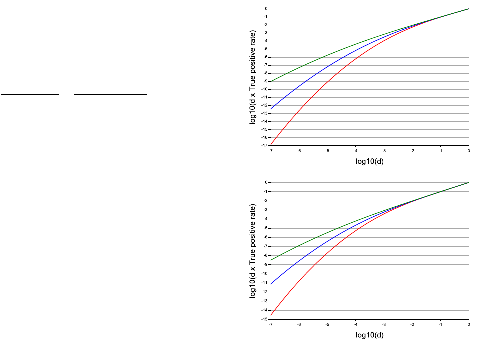
Figure 6: Fraction of population successfully at-
tacked (i.e., d · t
p
) vs. victim density, d, for clas-
sifiers shown in Figure 3. These curves used a
gain ratio of (a) G/C = 20, and (b) G/C = 100.
Observe that the fraction of users successfully
attacked always falls faster than density, and
generally far faster than density. For example,
when G/C = 100 and AUC=0.9 a factor of 10 re-
duction of d from 10
−5
to 10
−6
causes a factor of
1000 reduction in the fraction of the population
successfully attacked.
10

Figure 7: Country of claimed origin for 419
emails.
examples of many viable users, which are hard to find.
Ironically, for the attacker, more accurate classifiers
are much more easily built where they are least needed:
where victim densities are high. Figures 6 (b) shows
that even the worst classifier succeeds almost 1% of the
time when d = 10
−2
. The viable users found can then
be used to train and make the classifier even better.
However, when d = 10
−5
this same classifier succeeds
only over a portion 10
−8
of the population; i.e., it can
profitably find only a handful of victims in a population
of 200 million.
Thus, while it is plausible that an attacker might have
99.999% ability to distinguish viable users from non-
viable at high victim densities, it is almost impossible
to believe that this might be the case when d is low.
It’s hard to build algorithms that are very accurate at
detecting rare things, because rare things are, well, rare.
Faith that very accurate classifiers for very rare events
can be built without training data is generally confined
to those who are deluded, or have the luxury of never
putting their claims to the test.
4. DISCUSSION
4.1 Why do Nigerian scammers say that they
are from Nigeria?
An examination of a web-site that catalogs scam emails
shows that 51% mention Nigeria as the source of funds
[1], with a further 34% mentioning Cˆote d’Ivoire, Burk-
ina Faso, Ghana, Senegal or some other West African
country (see Figure 7). This finding is certainly sup-
ported by an analysis of the mail of this genre received
by the author.
Why so little imagination? Why don’t Nigerian scam-
mers claim to be from Turkey, or Portugal or Switzer-
land or New Jersey? Stupidity is an unsatisfactory an-
swer: the scam requires skill in manipulation, consid-
erable inventiveness and mastery of a language that is
non-native for a majority of Nigerians. It would seem
odd that after lying about his gender, stolen millions,
corrupt officials, wicked in-laws, near-death escapes and
secret safety deposit boxes that it would fail to occur
to the scammer to lie also about his location. That the
collection point for the money is constrained to be in
Nigeria doesn’t seem a plausible reason either. If the
scam goes well, and the user is willing to send money, a
collection point outside of Nigeria is surely not a prob-
lem if the amount is large enough.
“Nigerian Scam” is one of five suggested auto-completes
in a Google search for “Nigeria” (see Figure 8 retrieved
May 8, 2011). Thus, if the goal is to maximize response
to the email campaign it would seem that mentioning
“Nigeria” (a country that to many has b ecome syn-
onymous with scams) is counter-productive. One could
hardly choose a worse place to claim to be from if the
goal is to lure the unwary into email communication.
The scam involves an initial email campaign which
has almost zero cost per recipient. Only when poten-
tial victims respond does the labor-intensive and costly
effort of following up by email (and sometimes phone)
begin. In this view everyone who enters into email com-
munication with the scammer is “attacked” (i.e., engen-
ders a cost greater than zero). Of these, those who go
the whole distance and eventually send money are true
positives, while those who realize that it is a scam and
back out at some point are false positives.
If we assume that the scammer enters into email con-
versation (i.e., attacks) almost everyone who responds
his main opportunity to separate viable from non-viable
users is the wording of the original email. If the goal
is to attack as many people as possible, then the email
should be designed to lure as many as possible. How-
ever, we’ve seen that attacking the maximum number
of people does not maximize profit. Operating at the
OOP involves attacking only the most likely targets.
Who are the most likely targets for a Nigerian scam-
mer? Since the scam is entirely one of manipulation
he would like to attack (i.e., enter into correspondence
with) only those who are most gullible. They also need,
of course, to have money and an absence of any factors
that would prevent them from following through all the
way to sending money.
Since gullibility is unobservable, the best strategy is
to get those who possess this quality to self-identify. An
email with tales of fabulous amounts of money and West
African corruption will strike all but the most gullible
as bizarre. It will be recognized and ignored by anyone
who has been using the Internet long enough to have
seen it several times. It will be figured out by anyone
savvy enough to use a search engine and follow up on
the auto-complete suggestions such as shown in Figure
8. It won’t be pursued by anyone who consults sensible
11

family or fiends, or who reads any of the advice banks
and money transfer agencies make available. Those who
remain are the scammers ideal targets. They represent
a tiny subset of the overall population. In the language
of our analysis the density of viable victims, d, is very
low: perhaps 1-in-10,000 or 1-in-100,00 or fewer will fall
for this scam.
As we’ve seen, in Section 3.3, at low victim densi-
ties the attack/don’t attack decisions must be extremely
conservative. If only 0.00001% of the population is vi-
able then mistakenly attacking even a small portion of
the 99.999% of the population that is non-viable de-
stroys profit. The initial email is effectively the at-
tacker’s classifier: it determines who responds, and thus
who the scammer attacks (i.e., enters into email con-
versation with). The goal of the email is not so much
to attract viable users as to repel the non-viable ones,
who greatly outnumber them. Failure to repel all but a
tiny fraction of non-viable users will make the scheme
unprofitable. The mirth which the fabulous tales of
Nigerian scam emails provoke suggests that it is mostly
successful in this regard. A less outlandish wording that
did not mention Nigeria would almost certainly gather
more total responses and more viable responses, but
would yield lower overall profit. Recall, that viability
requires that the scammer actually extract money from
the victim: those who are fooled for a while, but then
figure it out, or who balk at the last hurdle are precisely
the exp ensive false positives that the scammer must de-
ter.
In choosing a wording to dissuade all but the like-
liest prospects the scammer reveals a great sensitivity
to false positives. This indicates that he is operating
in the far left portion of the ROC curve. This in turn
suggests a more precarious financial proposition than is
often assumed.
4.2 Putting false positives to work
We find that, when C > 0, the attacker faces a prob-
lem familiar to the rest of us: the need to manage the ra-
tio of false to true positives drives our decisions. When
this is hard he retreats to the lower left corner of the
ROC curve. In so doing he attacks fewer and fewer
viable targets. This is good news.
We now explore how we can make this even better
and exploit this analysis to make an attacker’s life even
harder. Great effort in security has been devoted to
reducing true positives. User education, firewalls, anti-
virus products etc, fall into this camp of trying to reduce
the likelihood of success. There has also been effort on
reducing G the gain that an attacker makes. These are
techniques that try to reduce the value of the stolen
goods; fraud detection at the back-end might be an
instance of reducing the value of stolen passwords or
credit cards. There has been some effort at increasing
Figure 8: Google search offering “Nigerian
Scam” as an auto-complete suggestions for the
string “Nigeria”.
C. Proposals to add a cost to spam, and CAPTHCHA’s
fall into this camp [6, 4]. Relatively unexplored is the
option of intentionally increasing
f
p
with the goal of
wasting attacker resources. If we inject false positives
(i.e., non-viable but plausible targets) we reduce the vi-
able target density. As we saw in Section 3.3 this causes
a deterioration in the attackers prospects and improves
the social good. If we can increase f
p
to the point where
the expected return in (1) becomes negative the attack
may be uneconomic.
It is, of course, entirely obvious that adding false
positives reduces the attacker’s return. Scam-baiters,
for example, who intentionally lure Nigerian scammers
into time-wasting conversations have this as one of their
goals [2]. What is not obvious, and what our analysis
reveals, is how dramatic an effect this can have. We
saw in Section 3.4 that a 10× reduction in density could
produce a 1000× reduction in victims found.
Inserting false positives effectively reduces the viable
victim density. Figure 6 reveals that the portion of
the population successfully attacked falls much faster
than victim density, and that this trend accelerates as
d decreases. For example, in Figure 6 (a) for the AUC=
0.9 classifier the 10× reduction in d from 10
−2
to 10
−3
produces a 45× reduction in d · t
p
, while the reduction
in d from 10
−5
to 10
−6
produces a 3500× reduction.
This reiterates that at low densities the attacker is far
more sensitive to false positives.
5. RELATED WORK
The question of tradeoffs in security is not a new
one. Numerous authors have pointed out that, even
though security is often looked at as binary, it cannot
escape the budgeting, tradeoffs and compromises that
12
are inevitable in the real world. The scalable nature
of many web attacks has been noted by many authors,
and indeed this has often been invoked as a possible
source of weakness for attackers. Anderson [18] shows
that incentives greatly influence security outcomes and
demonstrates some of the perverse outcomes when they
are mis-aligned. Since 2000 the Workshop on the Eco-
nomics of Information Security (WEIS) has focussed on
incentives and economic tradeoffs in security.
Varian suggests that many systems are structured so
that overall security depends on the weakest-link [13].
Gordon and Loeb [16] describe a deferred investment
approach to security. They suggest that, owing to the
defender’s uncertainty over which attacks are most cost
effective, it makes sense to “wait and see” before com-
mitting to investment decisions. Boehme and Moore
[20] develop this approach and examine an adaptive
model of security investment, where a defender invests
most in the attack with the least expected cost. Inter-
estingly, in an iterative framework, where there are mul-
tiple rounds, they find that security under-investment
can be rational until threats are realized. Unlike much
of the weakest-link work, our analysis focusses on the at-
tacker’s difficulty in selecting profitable targets rather
than the defender’s difficulty in making investments.
However, strategies that suggest that under-investment
is not punished as severely as one might think spring
also from our findings.
Grossklags et al.[12] examine security from a game
theoretic framework. They examine weakest-link, best-
shot and sum-of-effort games and examine Nash equi-
libria and social optima for different classes of attacks
and defense. They also introduce a weakest-target game
‘where the attacker will always be able to compromise
the entity (or entities) with the lowest protection level,
but will leave other entities unharmed.” A main p oint
of contrast between our model and the weakest-target
game is that in our model those with the lowest protec-
tion level get a free-ride. So long as there are not enough
of the to make the overall attack profitable, then even
the weakest targets escape.
Fultz and Grossklags [17] extend this work by now
making the attacker a strategic economic actor, and
extending to multiple attackers. As with Grossklags
et al.[12] and Schechter and Smith [21] attacker cost is
not included in the model, and the attacker is limited
mostly by a probability of being caught. Our model, by
contrast, assumes that for Internet attackers the risk of
apprehension is negligible, while the costs are the main
limitation on attacks.
In earlier work we offered a partial explanation for
why many attacks fail to materialize [14]. If the at-
tack opportunities are divided between targeted attack-
ers (who expend per-user effort) and scalable attackers
(who don’t) a huge fraction of attacks fail to be prof-
itable since targeting is expensive. This paper extends
this work and shows that even scalable attacks can fail
to be economic. A key finding is that attacking a crowd
of users rather than individuals involves facing a sum-
of-effort rather than weakest-link defense. The greater
robustness and well-known free-rider effects that accom-
pany sum-of-effort systems form most of the explana-
tion for the missing attacks. Florˆencio and Herley [9]
address the question of why many attacks achieve much
less harm than they seem capable of. Their model sug-
gests that an attacker who is constrained to make a
profit in expectation will ignore many viable targets.
Odlyzko [3] addresses the question of achieving secu-
rity with insecure systems, and also confront the para-
dox that “there simply have not been any big cyberse-
curity disasters, in spite of all the dire warnings.” His
observation that attacks thrive in cyberspace because
they are “less expensive, much more widespread, and
faster” is similar to our segmentation of broadcast at-
tacks.
While trade-off problems have been extensively stud-
ied not much work has examined the problem from an
attacker point of view. Dwork and Naor [6] examine the
question of increasing the cost of all attacks. They note
the danger of situations where costs are zero and sug-
gest various ways that all positives (not just false ones)
can be increased in cost. Their insight is that when
false positives outnumber legitimate use then a small
cost greatly interferes with attacks for minimal effect
on legitimate use. Schechter and Smith [21] investigate
various investment strategies to deter attackers who
face the risk of penalties when attacks fail. Ford and
Gordon [10] suggest enlisting many virtual machines in
botnets. These machines join the network, but refuse
to perform the valuable business functions (e.g., send-
ing spam) and thus make the value of the botnet less
predictable. Scambaiters [2] advocate wasting attacker
time. However this is done manually, rather than in
an automated way, and for sport rather than to reduce
their profitability.
6. CONCLUSION
We explore attack decisions as binary classification
problems. This surfaces the fundamental tradeoff that
an attacker must make. To maximize profit an attacker
will not pursue all viable users, but must balance the
gain from true positives against the cost of false posi-
tives. We show how this difficulty allows many viable
victims to escape harm. This difficulty increases dra-
matically as the density of viable victims in the pop-
ulation decreases. For attacks with very low victim
densities the situation is extremely challenging. Unless
viable and non-viable users can be distinguished with
great accuracy the vast majority of viable users must be
left un-attacked. However, building an accurate classi-
13
fier requires many viable samples. This suggests that
at very low densities certain attacks pose no economic
threat to anyone, even though there may be many vi-
able targets. Most work on vulnerabilities ignores this
fundamental question.
Thinking like an attacker is a skill rightly valued among
defenders. It helps expose vulnerabilities and brings
poor assumptions to light. We suggest that thinking
like an attacker does not end when a hole is found, but
must continue (as an attacker would continue) in deter-
mining how the hole can be monetized. Attacking as
a business must identify targets, and this is easy only
if we believe that attackers have solved a problem that
has vexed multiple communities for decades.
7. REFERENCES
[1] http://www.potifos.com/fraud/.
[2] http://www.419eater.com/.
[3] A. Odlyzko. Providing Security With Insecure
Systems. WiSec, 2010.
[4] L. Ahn, M. Blum, N. Hopper, and J. Langford.
Captcha: Using hard ai problems for security. In
Proceedings of the 22nd international conference
on Theory and applications of cryptographic
techniques, pages 294–311. Springer-Verlag, 2003.
[5] S. Axelsson. The base-rate fallacy and the
difficulty of intrusion detection. ACM
Transactions on Information and System Security
(TISSEC), 3(3):186–205, 2000.
[6] C. Dwork and M. Naor. Pricing via Processing or
Combatting Junk Mail. Crypto, 1992.
[7] D. Florˆencio and C. Herley. Is Everything We
Know About Password-stealing Wrong? IEEE
Security & Privacy Magazine. To appear.
[8] D. Florˆencio and C. Herley. Sex, Lies and
Cyber-crime Surveys. WEIS, 2011, Fairfax.
[9] D. Florˆencio and C. Herley. Where Do All the
Attacks Go? WEIS, 2011, Fairfax.
[10] Ford R., and Gordon S. Cent, Five Cent, Ten
Cent, Dollar: Hitting Spyware where it Really
Hurt$. NSPW, 2006.
[11] D. Geer, R. Bace, P. Gutmann, P. Metzger,
C. Pfleeger, J. Quarterman, and B. Schneier.
Cyber insecurity: The cost of monopoly.
Computer and Communications Industry
Association (CCIA), Sep, 24, 2003.
[12] J. Grossklags, N. Christin, and J. Chuang. Secure
or insure?: a game-theoretic analysis of
information security games. WWW, 2008.
[13] H. R. Varian. System Reliability and Free Riding.
Economics of Information Security, 2004.
[14] C. Herley. The Plight of the Targeted Attacker in
a World of Scale. WEIS 2010, Boston.
[15] J. Sunshine, S. Egelman, H. Almuhimedi, N. Atri
and L. F. Cranor. Crying Wolf: An Empirical
Study of SSL Warning Effectiveness. Usenix
Security, 2009.
[16] L.A. Gordon and M.P. Loeb. The Economics of
Information Security Investment. ACM Trans. on
Information and System Security, 2002.
[17] N. Fultz and J. Grossklags. Blue versus Red:
Toward a Model of Distributed Security Attacks.
Financial Crypto, 2009.
[18] R. Anderson. Why Information Security is Hard.
In Proc. ACSAC, 2001.
[19] R. Anderson. Security Engineering. In Second ed.,
2008.
[20] R. Boehme and T. Moore. The Iterated
weakest-link: A Model of Adaptive Security
Investment. WEIS, 2009.
[21] S. Schechter and M. Smith. How Much Security is
Enough to Stop a Thief? In Financial
Cryptography, pages 122–137. Springer, 2003.
[22] H. L. van Trees. Detection, Estimation and
Modulation Theory: Part I. Wiley, 1968.
14
