Extreme Events and Overreaction to News

Spencer Yongwook Kwon and Johnny Tang

∗

January 26, 2023

Abstract

The presence of both systematic under-and-overreaction to news in ﬁnancial mar-

kets is a major puzzle. We propose a systematic predictor of under-and-overreaction to

news: the extremeness of the associated distribution of fundamentals. Using a compre-

hensive database of corporate news events, we identify substantial heterogeneity in both

reactions to news and extremeness of fundamentals across types of corporate events. We

document overreaction to more extreme event-types, such as leadership changes, M&A,

and customer announcements, and underreaction to less extreme event-types such as

earnings announcements. We show this is consistent with diagnostic expectations, a

model of belief formation based on the representativeness heuristic. The model further

predicts greater trading volume holding ﬁxed fundamentals and more sensitive belief

changes to more extreme corporate events, which we conﬁrm in the data. We calibrate

our model and show that it quantitatively matches the key features in our data.

∗

Spencer Yongwook Kwon: Harvard Business School and Harvard University, ykw[email protected]. Johnny

Tang: Harvard University, [email protected]ard.edu. We thank Malcolm Baker, Nick Barberis, Francesca

Bastianello, Michael Blank, Pedro Bordalo, John Campbell, Nicola Gennaioli, Mark Egan, Paul Fontanier,

Xavier Gabaix, Robin Greenwood, Sam Hanson, Alex Imas, Yueran Ma, Peter Maxted, Josh Schwartzstein,

Kelly Shue, Andrei Shleifer, David Solomon (discussant), Jeremy Stein, Adi Sunderam, Paul Tetlock, and

seminar participants at Harvard, Yale, and the 2021 Spring NBER Behavioral Finance meeting for helpful

comments and feedback.

1 Introduction

How do stock prices react to news? There has been extensive evidence of both over- and

under-reaction in ﬁnancial markets. On one hand, investors tend to be overly optimistic

about the long-term prospects of ﬁrms that have experienced a period of sustained earnings

growth, which lead to long-run reversals (De Bondt and Thaler (1985), Cutler et al. (1991),

Lakonishok et al. (1994), La Porta (1996), Bordalo et al. (2019)). At a shorter horizon, in-

vestors may overreact to a range of corporate news (Antweiler and Frank (2006)), potentially

spurred by spikes in media coverage, investor interest, or sentiment (Da et al. (2011), Tetlock

(2007)). On the other hand, a large literature documents that prices can react sluggishly

to news and lead to drift following earnings announcements (Bernard and Thomas (1989)),

the underpricing of proﬁtable ﬁrms (Bouchaud et al. (2019)), and momentum (Chan et al.

(1996)).

The presence of both systematic over- and under-reaction is a major puzzle. Some skep-

tics view the variation in market reaction to news as random ﬂuctuations around the ra-

tional benchmark (e.g. Fama (1998)). In this paper, we oﬀer an alternative perspective by

proposing a systematic determinant of under-and-overreaction – the extremeness of funda-

mentals associated with the news. We show that a core feature of corporate news is that

the distribution of fundamentals is extreme: while most corporate news tend to have a rela-

tively immaterial impact on overall valuation, there are tail events with major implications

that signiﬁcantly shape investor reactions to future analogous news. We formally deﬁne

the extremeness of a type of news, or an event-type (e.g. earnings announcements) as the

tail-fatness (Gabaix (2009)) of the distribution of fundamentals. In other words, we deﬁne

extremeness to be a property of the whole event-type, rather than of a particular news event:

the more extreme the event-type, the greater the relative diﬀerence between the fundamen-

tals of its tail, e.g. the top 1% earnings announcements, to that of its typical event, e.g.

the median. We hypothesize that more extreme types of news are associated with greater

1

overreaction, as investors are relatively likelier to focus on the tail events when reacting to

news.

To formalize this intuition, we apply diagnostic expectations (DE) (Bordalo et al. (2018)),

a model of belief formation based on Kahneman and Tversky’s representativeness heuristic,

to the setting of reaction to corporate news. DE capture the insight that agents overrepresent

states of the world that have become likelier in light of news and have been used to model ex-

uberance in credit booms, overreaction in macroeconomic forecasts (Bordalo et al. (2020b)),

and closest to our setting, the overvaluation of ﬁrms with high long-term growth prospects

(Bordalo et al. (2019)). Relative to these papers, we highlight the role of extreme events in

investor reaction to news. Our model predicts that as the extremeness of the type of news

increases, tail outcomes become more representative in light of news. When the distribution

of associated fundamentals becomes more extreme than the distribution in the absence of

news announcements, diagnostic expectations of fundamentals overshoot the rational bench-

mark and lead to overreaction. Conversely, if the news is suﬃciently less extreme, events

associated with no change in fundamentals become more representative and overweighted,

which causes underreaction. Our application consequently yields both underreaction and

overreaction, whereas previous applications of DE have largely focused on overreaction.

To derive predictions regarding asset prices and trading behavior, we introduce DE agents

into a stylized asset pricing model, where agents receive idiosyncratic signals of the funda-

mentals. In reaction to an extreme type of news, the average beliefs of investors and asset

prices overreact. This leads to reversals when prices eventually return to the rational bench-

mark. Furthermore, as all investors overreact to their idiosyncratic signal, there is greater

disagreement between investors who receive diﬀerent signals, which leads to higher trading

volume holding ﬁxed fundamentals. Conversely, in response to a less extreme type of news,

beliefs underreact, which leads to drift and lower trading volume. Our model thus gener-

ates the key predictions that more extreme types of news have greater return reversals and

2

disagreement-driven trading volume.

1

In the second part of the paper, we empirically test the predictions of the model. First, we

conﬁrm that investor reaction to diﬀerent types of corporate news is highly heterogeneous.

Drawing from a comprehensive database of corporate news events in the US from 2011 to

2018, we ﬁnd not only post-announcement drift for events such as earnings announcements,

but also reversals for a wide range of event-types, including leadership changes, business

expansions, mergers, acquisitions, and customer-related events. Short-term overreaction to

news seems to be the norm across corporate events that do not frequently coincide with

earnings announcements.

2

The cross-section of drift and reversal across these types of news

is robust to diﬀerent measurement methods, such as estimation using portfolio sorts and a

full ﬁrm-day panel speciﬁcation, which accounts for overlapping returns and unconditional

market autocorrelations. We also show that the cross-section of drift and reversal is not

driven by sampling variation or non-event-driven forces.

We next measure the extremeness of the fundamentals and document signiﬁcant diﬀer-

ences across the news categories in our sample. Statistically, the extremeness of a news type

is captured by the fatness of the tail of the distribution of outcomes: the fatter the tail, the

farther the extreme, e.g. top 1%, events are from the median event. We measure extremeness

in several ways, with the Pareto tail index of power-law distributions being our preferred

measure.

3

We ﬁnd that the distribution of outcomes of an event-type, measured by realized

1

Our theory does not focus on why arbitrageurs cannot price out the distortions by trading against DE

agents. One of the reasons can be that by trading against potentially extreme events, the arbitrageurs are

taking on a negative skew-risk, which can command a signiﬁcant risk premium. Short-sale constraints on the

part of the arbitrageur in response to positive company news can also contribute to the limits of arbitrage.

To focus on the distortions due to investor psychology, we simplify the arbitrageur response by positing a

simple reduced-form asset demand function that captures these risk and capital concerns.

2

We have chosen 90 days as our main choice of horizon, as it approximately corresponds to the range of

post-earnings drift studies (e.g. Bernard and Thomas (1989)). Our ﬁndings are robust to the exact horizon

of the reversal (from 60 days to 3 months).

3

The Pareto tail index is given by the slope of the log-log rank-size regressions of event-day returns, also

known as power-law regressions (Gabaix (2016)). For power-law, or Pareto, distributions, this regression

precisely measures the tail fatness, also known as the Pareto index. The measurement of fat tails has received

recent attention in economics, from wealth distributions and city size, to stock market returns and trading

3

cash ﬂow growth, event-day returns, and longer-term returns, are very well described by the

fat-tailed power-law distribution, consistent with earlier ﬁndings (e.g. Gabaix (2016)), with

signiﬁcant variation in the Pareto tail index across event-types.

Equipped with these baseline results, we test the core asset-pricing predictions of our

model: more extreme event types are more overreacted to, with greater reversals and trading

volume. Consistent with our ﬁrst prediction, we ﬁnd that more extreme corporate event types

exhibit more post-announcement return reversals, whereas less extreme event types exhibit

more post-announcement drift. We estimate that fatter-tailed events exhibit reversals up

to 14% of the event-day return, while thinner-tailed events experience continued drifts of

up to 10% of the event-day return. We show that this pattern is robustly found across

return horizons and rule out alternative explanations such as familiarity or seasonality across

diﬀerent event-types. Turning to our second prediction, we conﬁrm that more extreme

corporate events have higher trading volumes conditional on the magnitudes of event-day

returns. Conditional on a 10% event-day return, we estimate that turnover for diﬀerent event-

types would range from 4.8% for the thinnest-tailed event-types to 6.3% for the fattest-tailed

event-types. This range of estimated conditional turnovers quantitatively matches the range

(4.6% to 7.0%) of the actual conditional turnovers across event-types we observe in our data.

To further validate the explanatory power of extremeness in under- and overreaction, we

turn to expectations data to directly measure how investor beliefs change in response to news.

We use stock analysts’ earnings per share (EPS) forecasts as a proxy for investor beliefs, and

we measure belief under- and overreaction using the Coibion and Gorodnichenko (2015)

methodology of comparing ex-post forecast errors to forecast revisions. Consistent with our

model, we ﬁnd evidence suggesting that analyst forecasts react more sensitively to more

extreme event types. The analysis allows us to move beyond trading data to provide further

volume. For a general reference, see Gabaix (2016). The extremeness of a distribution has been computed

using various alternative measures, ranging from quantile ratios to higher normalized moments such as skew

and kurtosis. In Section 4, we discuss the relative merits of each measures and conﬁrm that our results are

robust to the choice of a particular measure.

4

evidence consistent with beliefs playing a central role in explaining under- and overreaction

in asset prices.

We conclude with a calibration of our model to assess its explanatory power. We empir-

ically estimate the diagnostic parameter θ and generate model-implied price drift/reversal

and trading behaviors and compare these model-implied quantities to those we observe in

the data. We ﬁnd that the model-implied quantities quantitatively ﬁt the cross-sectional

variation in under- and overreaction in asset prices and in trading volumes across event

types, with the calibrated diagnostic parameter θ = 0.95 broadly in line with the estimates

obtained in earlier works (Bordalo et al. (2020b, 2019)).

Our paper relates to the extensive theoretical (Barberis et al. (1998), Hong and Stein

(1999), Daniel et al. (1998)) and empirical (De Bondt and Thaler (1985), Lakonishok et al.

(1994), La Porta (1996), Daniel and Titman (2006), Bernard and Thomas (1989), and Bor-

dalo et al. (2019)) literature studying investor over- and underreaction in asset pricing. A

large literature focuses on horizon as the key variation and documents short-term underreac-

tion and long-term overreaction in stock prices (Bernard and Thomas (1989), De Bondt and

Thaler (1985), Bordalo et al. (2019)) and in yield curves (Giglio and Kelly (2018)). Recent

work has also connected asset price over- and underreaction to expectations (Bordalo et al.

(2019); d’Arienzo (2020); Wang (2019)). While this research focuses on the variation in

horizon, we ﬁx the horizon to the short-term and focus on variations in the types of events.

In this sense, our work also relates to Daniel and Titman (2006), which ﬁnds evidence of

long-horizon overreaction to intangible information, Antweiler and Frank (2006), which ﬁnds

overreaction to a wider range of news, and Chang et al. (2017) and Hartzmark and Shue

(2018), which ﬁnd short-term investor overreaction to predictable seasonal components of

earnings and contrast to previous earnings. Relative to this work, we focus primarily on

explaining the variation in overreaction and underreaction across types of corporate news

through the lens of the extremeness of fundamentals.

Our work also relates to the growing literature that studies psychological foundations

5

of information processing and their applications to ﬁnancial settings. Overreaction has also

been attributed to extrapolation (Barberis et al. (2015, 2018)), cursedness (Eyster et al.

(2019)), and partial-equilibrium thinking (Bastianello and Fontanier (2019)). A related re-

cent literature also delves into fundamental mechanisms of memory in asset pricing (Wachter

and Kahana (2019); Nagel and Xu (2019)) and in an experimental context (Enke et al. (2020),

Bordalo et al. (2020a, 2021)). While our model also emphasizes the role of recall of extreme

outcomes in light of news, we focus on the variation in short-term asset price reactions to

speciﬁc news items across diﬀerent types of events.

Lastly, our work relates to the large literature on asset price reactions to news and

media coverage. Prior work on this topic has found that individual investors are prone to

buying attention-grabbing stocks which appear in the news (Barber and Odean (2008)).

Consistent with these ﬁndings, there is evidence of short-term overreaction driven by spikes

in investor interest and sentiment (Tetlock (2007), Da et al. (2011)), which can be spurred

partially by media coverage (Engelberg et al. (2012)). While media and investor sentiment

can generate short-term overreaction, our work connects investor attention and overreaction

to the fundamentals of the news. In our framework, investor attention is drawn to news that

bring to mind extreme outcomes in the past. Furthermore, our psychologically-motivated

framework points to extremeness as a measurable quantity which can explain the quantitative

variation in both under- and over-reaction.

The rest of the paper is organized as follows. Section 2 presents the model and discusses

its motivation in ﬁnancial narratives and psychology research. Section 3 describes the data.

Section 4 documents heterogeneity in the short-term reaction to diﬀerent corporate develop-

ments and identiﬁes signiﬁcant diﬀerences in the extremeness of the fundamental distribution

across diﬀerent event-types. Section 5 tests the main asset pricing predictions of the model,

linking extremeness of fundamentals to overreaction, validate our hypothesis on expectations

data, and provides a calibration of our model. Section 6 concludes.

6

2 Tail events and reaction to news

In this section, we apply diagnostic expectations (DE) to the setting of reactions to corporate

news announcements. We assume that the fundamentals associated with corporate news

follow an extreme distribution and that diﬀerent types of news are diﬀerently extreme. This

diﬀerence in the underlying fundamental distribution will be a key driver of the diﬀerences

in market reactions to news, with greater overreaction for more extreme types of news. We

revisit and verify these assumptions in the empirical section.

2.1 Diagnostic Expectations of Fundamentals

Let E be an event-type and λ be the fundamentals associated with an event of type E, which

is drawn from the distribution π(λ|E). Each investor i receives a noisy, idiosyncratic signal

s

i

drawn from a distribution f (s|λ). For simplicity, we assume that λ ≥ 0: the event has

positive impact. The negative case follows analogously.

We assume that the distribution of fundamentals for a given event-type follows a power-

law distribution:

π(λ|E) = ζ

−1

E

λ

ζ

−1

E

0,E

λ

ζ

−1

E

+1

for λ ≥ λ

0,E

.

4

(1)

There are two parameters of the distribution: λ

0,E

, the scale parameter, and 0 < ζ

E

< 1, the

tail parameter, which governs the extremeness of the distribution and varies across E: the

higher the ζ

E

, the more extreme the event-type. Upon the release of news, an agent i learns

of the event-type E and receives an idiosyncratic noisy signal s

i

of the latent fundamentals

4

For analytical tractability, we assume that the distribution of fundamentals has either positive or negative

support. This assumption can be given an intuitive framing if the investor interprets news according to both

its event-type and whether it is good or bad news. In practice, we ﬁnd that the extremeness of event-types

is similar for both good and bad news, which motivates us to make the above simplifying assumption.

7

λ. We assume that s

i

is drawn from the conjugate distribution:

s

i

= λ · u

i

, u

i

∼ Unif[0, 1].

5

(2)

Then, the rational posterior distribution of fundamentals given (E, s

i

) are given by:

π(λ|E, s

i

) = (ζ

−1

E

+ 1) ·

λ

ζ

−1

E

+1

1,E

λ

ζ

−1

E

+2

for λ ≥ λ

1,E

= max{s

i

, λ

0,E

}. (3)

We assume that investors form diagnostic expectations of fundamentals given news (Bor-

dalo et al. (2018)), such that the posterior distribution of fundamentals is given by:

π

θ

(λ|E, s

i

) ∝ π(λ|E, s

i

) ·



π(λ|E, s

i

)

π(λ|No News)



θ

. (4)

The likelihood ratio

π(λ|E,s

i

)

π(λ|No News)

reﬂects the representativeness of fundamentals λ given the

news (E, s

i

), relative to the common benchmark π(λ|No News), the distribution of funda-

mentals that would prevail in the absence of news. The parameter θ reﬂects the degree

to which more representative fundamentals are overweighted, with θ = 0 corresponding to

the rational case. In this sense, DE capture the psychology that investors overweight the

probability of outcomes that have become likelier in light of news.

6

5

This can be generalized to a sub-class of the Beta distribution: f(s|θ) = γ ·

s

γ−1

θ

γ

.

6

In general, diagnostic expectations are motivated by Kahneman and Tversky’s representativeness heuris-

tic, the psychological tendency to overrepresent representative attributes of a class, where “an attribute is

representative ... if ... the relative frequency of this attribute is much higher in that class than in a reference

class” (Tversky and Kahneman (1983)). In other words, agents overestimate a trait t that is representative

of group G compared to a reference group −G:

π

θ

(t|G) ∝ π(t|G) ·



π(t|G)

π(t| − G)



θ

For example, in the context of stereotypes, the trait t = red hair is representative of G = Irish compared to

−G = rest of the world, and is overestimated. In the context of news and expectation formation, Bordalo

et al. (2018) set G as the arrival of new information and −G as the counterfactual in which no news arrives,

where the realized signal is equal to its ex ante expected value.

8

Following Bordalo et al. (2019, 2020b), we deﬁne the No-News distribution,

π(λ|No News), as the distribution of fundamentals in the absence of an event, conditional

on the idiosyncratic signal s

i

equal to its ex ante expected value. In other words, we ﬁrst

let π

d

(λ) be the distribution of fundamentals in the absence of any news announcement. We

assume that this distribution is symmetric around 0, with the tails of the distribution also

following a power-law:

π

d

(λ) =











π

0

(|λ|) for |λ| < λ

0,d

C · |λ|

−(ζ

−1

d

+1)

for |λ| > λ

0,d

,

with 0 < λ

0,d

≤ λ

0,E

for all event-types E. π

d

(λ) captures the movement in valuation unre-

lated to any particular announcement (e.g. Cutler et al. (1988), Savor (2012)). Furthermore,

we assume the tails of π

d

are also fat with tail index ζ

d

. This assumption is made not only

for analytical tractability, but also reﬂects a key feature of the data, that the distribution

of unconditional fundamentals, even outside of news-announcement days, has a fat tail (e.g.

Gabaix et al. (2003), Plerou et al. (1999), and Oh and Wachter (2018)). Then, the No-News

distribution is given by:

π(λ|No News) = π

d

(λ|s

i

= 0). (5)

Applying Equation 5 to Equation 4 gives the following characterization of investor beliefs in

reaction to an event of type E.

Proposition 1 (Diagnostic expectations with extreme fundamentals). The diagnostic ex-

pectations of fundamentals is given by:

E

θ

[λ|E, s

i

] = ψ(ζ

E

, ζ

d

, θ) · E[λ|E, s

i

] =

1 + ζ

E

+ θ



1 −

ζ

E

ζ

d



1 + ζ

E

+ (1 + ζ

E

) · θ



1 −

ζ

E

ζ

d



· E[λ|E, s

i

], (6)

where E[λ|E, s

i

] is the rational expectations. The distortion term ψ(ζ

E

, ζ

d

, θ) is increasing

9

in ζ

E

, with diagnostic expectations overreacting (ψ > 1) if and only if ζ

E

> ζ

d

.

0.03 0.04 0.05 0.06 0.07 0.08

0 20 40 60 80 100 120

Fundamentals

Density

Reference

Rational

Diagnostic

(a) DE, more extreme event-type

0.030 0.035 0.040 0.045 0.050 0.055 0.060

0 20 40 60 80 100 120

Fundamentals

Density

Reference

Rational

Diagnostic

(b) DE, less extreme event-type

Figure 1: Diagnostic expectations and the under-overreaction

Note: Figures 1a and 1b show the DE distortions of subjective fundamentals for more and less

extreme event-types, respectively. The solid red and blue curves plot the density functions

of the distributions of subjective fundamentals under diagnostic expectations. The solid

black curves plot the density functions under the rational distributions. The dotted black

curves plot the reference distributions. The solid black vertical lines plot the expectation of

fundamentals for the rational agents. The solid red and blue vertical lines plot the subjective

expectations of fundamentals for the diagnostic agents.

Figure 1 illustrates how DE distorts the expectations of fundamentals. In the left panel,

the fundamentals associated with event-type E is more extreme than what one may expect

from unconditional stock price ﬂuctuations: the rational posterior, in the solid black curve,

has a fatter tail than the reference distribution, in the dotted curve. In this case, diagnostic

expectations, shown in the red curve, further exaggerate the prevalence of extreme events,

causing the posterior mean to overshoot. On the other hand, if the event-type E is less

extreme relative to the reference distribution, the prevalence of extreme outcomes becomes

10

less likely in light of news. Consequently, diagnostic investors exaggerate this diﬀerence,

with the diagnostic posterior mean undershooting the rational benchmark.

The combination of diagnostic expectations with variation in fundamental extremeness

can help explain the cross-section of under-overreaction across event types. If news increases

the probability of extreme outcomes relative to the reference distribution, diagnostic agents

overestimate the probability of a tail outcome and overreact. This is similar to the intuition

given in Bordalo et al. (2019) – in response to news that signiﬁcantly increases the long-term

growth prospects of a company, investors exaggerate the probability that the company will

become “the next Google”. On the other hand, diagnostic expectations can also generate

underreaction if the underlying fundamental distribution is suﬃciently less extreme. While

a news may have a positive impact on valuations, if the distribution of potential outcomes

is less extreme than the reference distribution, expectations undershoot. Intuitively, agents

reason that while the event may be good news, it is less signiﬁcant relative to other extreme

outcomes they have seen in the market, leading to underreaction.

2.2 Asset pricing predictions

We now apply our model of expectations to a simple asset market setting, and derive implica-

tions for price, post-announcement drifts and reversals, and volume. We make the following

standard assumptions regarding the asset market. At t = 1, an event of type E and fun-

damentals λ occurs, with each agent i receiving an idiosyncratic signal of fundamentals,

s

i

= λ · u

i

. Based on their signal, each agent has a linear demand for the asset based on their

subjective fundamentals:

7

D

DE

i

(s

i

, p) = κ ·



E

θ

[λ|s

i

] − p



.

7

This can be justiﬁed from a standard mean-variance utility.

11

The price p

1

adjusts to clear the asset market, where we assume that the asset is in

zero net supply. As is standard, we also deﬁne the total trading volume to be V ol =

1

2



R

|D

i

(s

i

, p)|ds

i



, or half of the average absolute asset holdings in the economy. For nota-

tional simplicity, it is also convenient to deﬁne ζ

−1

θ,E

= ζ

−1

E

+ θ



ζ

−1

E

− ζ

−1

d



, where ζ

θ,E

> ζ

E

if

and only if ζ

E

> ζ

d

. Using these assumptions, one can derive the expression for price impact

and resulting volume of an event with fundamentals λ.

p

1

= (1 + ζ

θ,E

) ·

λ

2

0,E

+ λ

2

2λ

V ol =

1

2

κ · (1 + ζ

θ,E

) ·



λ

2

− λ

2

0,E

2λ



2

(7)

We assume that at t = 2, prices revert back to the rational benchmark, p

2

= (1 + ζ

E

) ·

λ

2

0,E

+λ

2

2λ

. In other words, the short-term price response to event E is given by the initial diag-

nostic price response p

1

, followed by the eventual drift or reversal to the rational benchmark

p

2

. This assumption is consistent with earlier ﬁndings which document excited, news-driven

investors initially entering the market (Barber and Odean (2008)), with arbitrageur capital

bringing prices back to rationality after a delay (Duﬃe (2010)). Eventually, at t = 3, the

long-run fundamentals λ are revealed. Note that p

2

6= λ: while the true fundamental may

be revealed to the investors in the long-run, it is unlikely to do so in the short-term, which

corresponds to our main empirical speciﬁcation.

One can deﬁne the theoretical drift-reversal coeﬃcients as:

β

E

=

p

2

− p

1

p

1

=

ζ

E

− ζ

θ,E

1 + ζ

θ,E

. (8)

β

E

is positive if p

1

undershoots p

2

and the market initially underreacts to the event. Con-

versely, if the market initially overreacts to the event and p

1

overshoots p

2

, β

E

is negative.

Figure 2 shows the relationship between β

E

and ζ

E

. Consistent with Proposition 1,

there is aggregate underreaction and drift, or β

E

≥ 0, if ζ

E

< ζ

d

: event-types that are less

12

0.25 0.30 0.35 0.40 0.45 0.50

−0.25 −0.20 −0.15 −0.10 −0.05 0.00 0.05

Fundamentals

Drift / Reversal

ζ

d

(a) Drift-Reversals vs Extremeness

0.25 0.30 0.35 0.40 0.45 0.50 0.55

0.006 0.007 0.008 0.009 0.010 0.011

Extremeness (zeta)

Volume

Rational

DE

(b) Volume vs Extremeness

Figure 2: DE predictions: over- and under-reaction, volume, and extremeness

Note: Figure 2a plots the theoretical relationship between stock price drift/reversal and the

extremeness of the distribution of fundamentals. The dashed vertical line (ζ

d

) corresponds

to the extremeness of the distribution of fundamentals for the reference distribution. Figure

2b plots the theoretical relationship between trading volume and the extremeness of the

distribution of fundamentals for rational agents in black and for DE agents in red.

extreme than the reference distribution are underreacted to. Conversely, if E is suﬃciently

extreme, ζ

E

> ζ

d

, the market overreacts to the event-type, resulting in reversals, i.e. β

e

≤ 0.

Furthermore, as depicted on the right panel of Figure 2, our theory also has implications for

the aggregate trading volume, holding ﬁxed fundamentals λ. Intuitively, as the underlying

fundamental distribution grows more extreme, diagnostic agents trade more aggressively

based on their private signals, leading to greater trading volume. While this relationship

is also true for the rational case, the dependence of volume on fundamental extremeness is

much more subdued relative to the diagnostic case.

The following proposition summarizes the above insights.

Proposition 2. 1. The drift-reversal coeﬃcient β

E

decreases in ζ

E

and the diagnostic

13

parameter θ. In particular, event-types whose distribution of fundamentals are more

extreme than the reference distribution (ζ

E

> ζ

d

) are associated with reversals. Con-

versely, event-types that are less extreme (ζ

E

< ζ

d

) are associated with drift.

2. The extremeness of the distribution of the short-term price movement, ζ(p

1

; E), in-

creases with the extremeness of the fundamentals ζ

E

.

3. Holding fundamentals λ ﬁxed, the total trading volume increases in ζ

E

.

The result that the extremeness of the short-term price movement is tightly linked with

the extremeness of fundamentals serves not only as a prediction of independent interest, but

also as a way to motivate our main empirical speciﬁcation. The extremeness of event-day

returns can be measured at a much higher frequency immediately following the news, in

contrast to the distribution of realized fundamentals, which are measured at a much lower

frequency and farther removed from the actual announcement. Proposition 2.2 allows us

to proxy the extremeness of event-type E with the more precisely measured extremeness of

event-day returns

ˆ

ζ(p

1

; E). Nonetheless, we show that our results are robust to alternative

proxies, including directly the extremeness of fundamentals.

To summarize, we make the following testable predictions regarding under-and-

overreaction to corporate news:

Prediction 1. Event-types with fatter-tailed distributions of fundamentals are associated

with greater price reversals. Conversely, event-types with thinner-tailed distributions of

fundamentals are associated with less reversal and greater drift.

Prediction 2. More extreme event-types are associated with greater trading volume, holding

ﬁxed the fundamentals of the event.

The core insight that generates our prediction is very simple: if over- and under-reaction

to news are driven by the propensity, or lack thereof, of tail outcomes to disproportion-

14

ately come to mind, then measuring exactly how extreme these tail outcomes are is key to

understanding the degree of over-and-underreaction to news.

2.3 Alternative explanations

Diagnostic expectations, when applied to corporate news with extreme fundamentals, provide

a natural way to understand the variation in how the market reacts to news. The model

predicts that news associated with more extreme distribution of fundamentals are tied to

greater overreaction, reversals, and trading volume. In this section, we discuss a number of

closely related alternative mechanisms that can also generate some of our core predictions.

Availability of extreme events

As evidenced by a rich literature on availability (Tversky and Kahneman (1973), Kahneman

(2011)), extreme tail events are dominantly available and have an outsized inﬂuence.

8

For

example, applying a simple probability weighting function (Kahneman and Tversky (1979))

that over-weights the probability of rare tail events would generate overreaction that is

increasing in the extremeness of the underlying distribution of fundamentals.

While this approach is also psychologically well-founded and can generate our core in-

tuition, it has a few limitations. First, in its simplest formulation, this model states that

tail events are always available, rather than being available in light of news. Second, the

over-representation of tail events always leads to over-reaction. In contrast, diagnostic ex-

pectation emphasizes the contrast between the distribution in light of the news to a reference

distribution, which not only leads to over-representation of tail events conditional on news,

but also leads to the full spectrum of over-and-underreaction.

8

Malmendier and Nagel (2011) and Knüpfer et al. (2017) document life-long impacts that experienced

economic depressions have on individuals’ investment and consumption choices.

15

Overconﬁdence and noisy information

Diﬀerent types of news may vary in their informativeness, or the “weight” of the associated

signals. For example, earnings announcements may be much more informative about the

future valuation of the company, while a CEO ﬁring may have much more uncertain impli-

cations for the future of the ﬁrm. If individuals insuﬃciently regard the weight of the signal,

they will underreact to informative news and overreact to less informative news (Griﬃn

and Tversky (1992)). This is in line with Solomon (2012), who documents that soft, and

potentially noisy, information can be spun in a positive way, leading to investor overreaction.

If more extreme event-types are also those associated with greater ambiguity or unin-

formative signals, this mechanism can also generate our predictions. A major challenge

for accounting for this explanation is that the degree of informativeness of news is diﬃcult

to measure empirically. In Section 5, we test this hypothesis by proxying for the unin-

formativeness of the signal with the average trading volume conditional on a given level of

fundamental news and ﬁnd that the explanatory power of fundamental extremeness is robust

to this alternative mechanism.

General drivers of investor attention

Tetlock (2014) points to the centrality of investor attention in driving short-term overreac-

tion, with attention-grabbing yet “uninformative media content” eliciting overreaction and

“informative content” otherwise eliciting underreaction. Our framework provides a psycho-

logical foundation for why investor attention to certain content can lead to over- and under-

reaction: if news coverage creates an association between a current event and past outcomes

that are more extreme, investors would overreact. Our model focuses on the simplest driver

of such an association, where extreme outcomes are likelier to come to mind if the distribu-

tion of fundamentals belonging to the same news type (e.g. past leadership changes) is more

16

extreme relative to the reference distribution.

9

Alternative explanations of underreaction

While DE predicts underreaction for types of news that are less extreme than the refer-

ence distribution, the extensive literature on PEAD documents many other potential causes

for underreaction. For instance, investors may be inattentive or face information frictions

unrelated to the distribution of underlying fundamentals (DellaVigna and Pollet (2009), En-

gelberg (2008)). Alternatively, institutional frictions, such as sluggish capital (Duﬃe (2010))

may dampen short-term price reaction to news. While we do not rule out these other im-

portant drivers of overall underreaction, we focus on what drives the diﬀerences in market

reaction across diﬀerent event-types through the lens of the the distribution of fundamentals.

3 Data

We use two main datasets for our news events and stock prices. First, we compile our list

of corporate news events from the Capital IQ Key Developments. The Capital IQ dataset

tracks major corporate news events such as earnings announcements, product and client

announcements, lawsuits/legal issues, leadership changes, and mergers and acquisitions, but

excludes macroeconomic news announcements such as interest rates and unemployment rates

that may aﬀect stock price returns. Among the corporate events in our dataset, we identify

the universe of events associated with US companies listed on a major US stock exchange

(NASDAQ, NYSE, and AMEX) that occurred between 2011 and 2018. Second, we obtain

daily stock returns and trading volume from CRSP, which we merge onto the Capital IQ

dataset.

As noted by the market microstructure literature, short-term price reversals can occur

9

In particular, we abstract away from any non-fundamental determinants of associations, such as general

features of similarity between the event and past extreme events.

17

due to liquidity concerns: at extremely short time scales, bid ask bounces generate negative

return autocorrelation. Even at longer time scales, there may be transient price pressure

as market makers demand compensation for liquidity while trading against uninformed ﬂow

(Kyle (1985), Nagel (2012)). To ameliorate these concerns, we exclude small-cap stocks from

our main analysis, which we deﬁne to be companies that have less than 2 billion dollars in

market capitalization at the time of the event.

10

Event types

We focus our analysis on news events that pertain to the real economic activities of the ﬁrm,

in particular its corporate and business operations, to ﬁlter out extraneous event-types.

In other words, we wish to use events that have direct relevance to the ﬁrm’s valuation

and its expected future cash ﬂows. As such, we select event types based on the following

methodology: ﬁrst, we select event types that have happened at least 1000 times across

all US companies in our sample between 2011 and 2018. Second, to focus on news related

to the fundamental operations of the ﬁrm, we exclude administrative events (such as name

changes and address changes)

11

, capital structure changes (such as debt and equity issuances

including IPOs

12

and SEOs), or trading activities, such as index exclusion, delisting, and

delayed SEC ﬁlings. Appendix B provides the full list of event types and which are included

and excluded in our main analysis.

Our ﬁnal universe of events comprise of 24 diﬀerent major event-types, including earnings

announcements, mergers and acquisitions, leadership changes, product and client-related

announcements, labor activities, and business reorganizations. The list of event-types we

use in our analysis is shown in Table 1. While we focus our main analyses on these events,

10

We repeat our analysis for the small-cap sample, and qualitatively replicate our main ﬁndings.

11

We note that some administrative events, such as announcements of earnings dates, or even name

changes, could be value-relevant for the ﬁrm. As a robustness check, we test our main empirical predictions

with the full set of events and obtain similar results.

12

We exclude IPOs in particular to avoid conﬂating IPO event day returns with the IPO premium.

18

we conduct robustness checks on the full sample of event types and show that our results

are robust to the precise inclusion/exclusion criteria that we employ.

Summary statistics

Table 1 reports summary statistics of the events in our sample. In general, corporate an-

nouncement days are characterized by signiﬁcant price movements and trading behavior.

The unconditional means across all the event-types are largely centered around zero with

a small but notable positive mean: with the exception of lowered earnings guidance, most

event-types are associated with a small positive daily return.

Corporate event days also tend to matter for stock prices: the standard deviation of

returns on the event days for almost all event-types exceed 2.1%, which is the average daily

return volatility of stocks in our sample. There is also meaningful variation in stock price

movements across event types. Earnings announcements and calls, credit rating downgrades,

and leadership changes tend to have higher absolute daily moves, while annual general meet-

ings, credit rating conﬁrmations, and CFO changes tend to have lower absolute daily moves.

In addition to returns, event days are also characterized by high trading volume. There

is also meaningful variation in the higher moments of the event day returns for the diﬀer-

ent event-types. As we explore in later sections, both the fundamentals and the event-day

returns associated with most event-types are fat-tailed, or extreme.

13

Are news announcement days separate?

Given the regularity of earnings announcements, one potential concern may be that the an-

nouncement dates in our sample largely coincide with the major earnings announcements.

The literature on strategic corporate announcement documents evidence of corporations

strategically timing their announcements, such as bunching multiple news events together

13

We introduce our measure of extremeness, given by the power-law exponent, in Section 4.

19

(e.g. Graﬃn et al. (2011)). If corporate events signiﬁcantly co-occur with earnings announce-

ments, isolating the component of event day return attributable to earnings announcement

from the eﬀects of other concurrent events could be challenging.

Table A2 presents the percentage of event occurrences in each event-type that overlaps

with an earnings announcement of the same ﬁrm. The results suggest that while some cor-

porate announcements are indeed concurrent with earnings announcements, a vast majority

of events occur on diﬀerent dates: 16 of the 24 event-types had less than half of their events

occurring on earnings announcement days. In fact, for most of these major events, over 90%

of these announcements do not occur on earnings announcement days.

4 Event-Type Heterogeneity

In this section and the next, we take our model to the data. We document three sets of

ﬁndings. First, the market reacts heterogeneously to diﬀerent types of news events. Second,

the distributions of fundamentals vary in their extremeness across event types. Third, con-

sistent with the core predictions of our model, event types with more extreme fundamentals

experience overreaction and greater trading volumes, while event types with less extreme

fundamentals experience underreaction and lower trading volumes.

4.1 Heterogeneous price reaction to corporate announcements

We ﬁrst document signiﬁcant heterogeneity in the stock price reactions to corporate news.

14

We estimate return autoregressions (e.g. Campbell et al. (1993)) and ﬁnd that while stock

14

These ﬁndings relate to prior work in the event-studies literature that jointly study a wider array of

corporate events. Antweiler and Frank (2006) classiﬁes WSJ articles into various corporate event types, and

documents overall overreaction. Neuhierl et al. (2013) studies corporate press releases and documents higher

return volatility and uncertainty post-announcements, and also ﬁnds reversals for a few event types such as

management changes and corporate restructuring. Relative to both works, our paper quantiﬁes the degree

of over-and-underreaction and highlights systematic diﬀerences across event types. Most importantly, our

paper documents variation in the extremeness of the fundamentals across diﬀerent event types, and shows

that it can explain the variation in over- and underreaction to news.

20

prices following earnings announcements exhibit post-announcement drift, many other types

of corporate events such as mergers, acquisitions, client announcements, and leadership

changes have post-announcement reversals. In fact, the majority of corporate events that do

not coincide with earnings announcements display reversals, with the economic magnitudes

of the reversals comparable to that of PEADs. We conduct robustness exercises and show

that the drift and reversal patterns are unlikely to be generated by sampling variation or

non-event-driven market dynamics, such as unconditional stock price autocorrelations, and

are robust to industry eﬀects and alternative return measures.

4.1.1 Cross-section of return drift and reversal

We ﬁrst present evidence of heterogeneity of drifts and reversals across corporate event

types by estimating return autocorrelation regressions. For each corporate event type e, we

estimate:

r

e,c,t+1,t+k

= α

e

+ β

e

· r

e,c,t,t+1

+ 

e,c,t

, (9)

where each observation is an occurrence of a corporate event of type e to company c at date

t. r

e,c,t+1,t+k

is the cumulative stock return following the event from date t + 1 to date t + k,

where days are restricted to trading days, and r

e,c,t,t+1

is the event-day stock return on date

t.

15

β

e

, our measure of interest, reﬂects the degree of return drift/reversals of event type e.

If β

e

= 1, then half of the price movements are realized on the event day on average, with a

predictable drift of equal proportion over the next k days. If β

e

= 0, excess returns are on

average not predictable by event-day returns, as implied by rational expectations. Finally,

if β

e

= −1, event-day returns are on average fully reversed. We set k = 90 trading days

for our baseline speciﬁcation of the stock price drift/reversal horizon, similar to the horizon

15

For example, let e be earnings announcements, c be Apple Inc., t be November 1st, 2018, and k be 90

days. Then the regression captures the relationship between the cumulative logarithmic return to Apple

stock price from November 1st, 2018 to 90 trading days in the future (March 18th, 2019), and the Apple

stock return on the day of November 1st, 2018.

21

considered by the PEAD literature.

16

We benchmark stock price returns relative to the S&P

500 returns and repeat our analysis without benchmarking as robustness checks. To ensure

our β

e

estimates are not driven by outliers, for each event type, we winsorize events at the

1% level. Standard errors are computed to account for cross-sectional and serial correlations

in the error term.

Figure 3: Reversal vs Drift

Note: Figure 3 plots the estimated β

e

for each of the 24 event types corresponding to eq.

(9).

Figure 3 plots the estimated β

e

coeﬃcients and Table 2 reports the estimates numerically.

Notably, the β

e

estimates exhibit considerable variation across diﬀerent types of events. In

particular, 11 out of the 24 event types in our sample exhibit post-announcement reversals.

While we ﬁnd positive return autocorrelation indicating post-announcement drift for earnings

16

We also set k = 30, 60, and 120 as robustness checks and obtain qualitatively similar results.

22

announcements, we also ﬁnd meaningful reversals for other corporate event types, including

leadership changes, mergers and acquistions, and client-related announcements. Table 2 also

reports the standard errors corresponding to individual β

e

estimates and we ﬁnd that seven

of the individual β

e

estimates are statistically distinguishable from zero at the 5% level.

These event types are among the most common event types in our sample. To evaluate

the overall statistical signiﬁcance of post-announcement drifts and reversals, we estimate a

pooled version of eq. (9) across all event types e:

r

e,c,t+1,t+k

= α + β

e

· 1(Event

e

) · r

e,c,t,t+1

+ 

e,c,t

, (10)

where each observation is a corporate event, and 1(Event

e

) is a dummy variable for event

type e. The joint F-statistic of the pooled speciﬁcation is 1.79, which strongly rejects the null

hypothesis that the event type-speciﬁc β

e

’s are jointly zero (p < 0.01). An analogous test also

strongly rejects the null hypothesis that the β

e

’s are jointly equal (F = 1.85, p < 0.01) As

such, the analysis indicates signiﬁcant variation in post-announcement drifts and reversals

in stock prices.

To interpret the economic magnitudes of the post-announcement drifts and reversals,

we construct sorted portfolios based on the event-day returns for each type of corporate

news. We divide our event types into two types based on the overlap of each event type

with earnings announcements. We deﬁne an event type as earnings-overlapping if more

than 50% of the events of the event type occur within a 5-day window around the same

ﬁrm’s earnings announcements and non-earnings-overlapping otherwise. Table A2 reports

each event type’s overlap with earnings announcements, which is bimodal: certain types of

news are frequently announced around earnings announcements, including announcements

of operating results, dividends, and corporate guidances, while other types of news, such

as mergers and acquisitions, client and product announcements, and legal issues, are rarely

announced around earnings announcements. For each of the two categories, we sort all events

23

within the category by their event-day returns and create ten sorted portfolios based on the

event-day returns. For example, portfolio 1 in each category represents the 10% of events

that had the lowest event-day returns and portfolio 10 represents the 10% with the highest

event-day returns. We calculate the cumulative returns to an equal-weighted winner-minus-

loser trading strategy that buys portfolio 10 and sells portfolio 1, which delivers positive

cumulative returns for events with post-announcement drifts and negative for reversals.

Figure 4: Sorted Portfolios of Earnings-Overlapping vs. Non-Earnings-Overlapping Events

Note: Figure 4 plots the cumulative abnormal returns to winner-minus-loser strategies for

sorted portfolios created on earnings-overlapping events (blue) and non-earnings-overlapping

events (red). The stocks are sorted based on the event-day returns into ten equally-sized

portfolios. The winner-minus-loser strategy buys the portfolio with the highest event-day

returns and shorts the portfolio with the lowest event-day returns.

24

Figure 4 presents the results. Consistent with Bernard and Thomas (1989) and the

PEAD literature, for earnings-overlapping events, a top-minus-bottom strategy generates

128 basis points of cumulative returns over a 90 day period. On the other hand, for non-

earning-overlapping events, the same strategy loses 46 basis points over a 90 day period.

The evidence thus suggests that while post-announcement drift occurs for earnings, post-

announcement reversals of a slightly lower but comparable magnitude are prevalent for other

event types.

4.1.2 Robustness exercises

We now conduct a series of robustness checks to test for alternative hypotheses that could

generate our results.

A. Full ﬁrm-day panel speciﬁcation to account for unconditional market au-

tocorrelations and event overlap

We present a panel speciﬁcation for our results to address two potential concerns. First,

not all corporate events occur at regularly scheduled intervals, so the event windows that

we study could contain overlapping event windows across diﬀerent events. For instance, if a

ﬁrm changed their CEO on October 1 and then announced their earnings on October 31, the

period immediately after the earnings announcement on October 31 would also be contained

in the event window for the CEO change. Another potential concern is that our results

may be driven by unconditional market dynamics unrelated to corporate news, for example

due to unconditional reversals to large returns (Chan (2003)). Then event types with larger

event-day returns may mechanically experience more post-event reversals and not because

market participants overreact more to those event types.

To address these two sets of concerns, we estimate our return autoregression in a panel

speciﬁcation. We construct a full ﬁrm-day panel where the observations are all ﬁrm-days over

the entire sample period. This ensures that the return of each ﬁrm on each day is sampled

25

only once and also accounts for overlapping news events that occur to the same ﬁrm over

the same time period, thus mitigating the overlapping observations concern. To account

for unconditional market return autocorrelations, we ﬂexibly control for the unconditional

market response to non-event-day returns. Our panel regression speciﬁcation is as follows:

r

c,t+1,t+90

= α + f(r

c,t

) +

X

e∈E

β

e

· 1(e

ct

) · r

c,t

+ 

ct

, (11)

where 1(e

ct

) is an indicator variable for whether a corporate event of type e occurred for ﬁrm

c on day t.

17

The term f(r

c,t

) captures the component of future market returns predictable

by unconditional returns, regardless of whether it is due to a particular event type. β

e

therefore identiﬁes the drift and reversal attributed to event type e in excess of the component

predictable by unconditional returns. We compute standard errors following Driscoll and

Kraay (1998) to account for overlaps and autocorrelated errors. We implement two versions

of f(r

c,t

). First, we set f (r

c,t

) = γ · r

c,t

, with γ capturing the unconditional drift or reversals.

Second, to address potential non-linearities in the autocorrelation of unconditional returns,

we set f(r

c,t

) =

P

10

i=1

γ

i

· 1(r

c,t

∈ ∆

i

), where 1(r

c,t

∈ ∆

i

) is an indicator variable for whether

r

c,t

is in the i-th decile of event-day returns.

Table A5 reports the corresponding results. Across all speciﬁcations, we ﬁnd that the

heterogeneity in the cross-section of drift and reversal to diﬀerent types of corporate events

are quantitatively consistent across speciﬁcations controlling for event-day returns. The β

e

estimates in the full ﬁrm-day panel regression range from 0.41 to -0.38 (based on the non-

parametric speciﬁcation of f), and are quantitatively similar to our previous β

e

estimates

from eq. (9). Overall, the results of the ﬁrm-day panel speciﬁcation with ﬂexible event-

day return controls suggest that our β estimates are robust to overlapping observations and

reﬂect true heterogeneity in responses to diﬀerent event types.

17

To avoid potential collinearities, the set of events E excludes event types that co-occur within ﬁve days

of earnings announcements at least 50% of the time, so there are 17 total event type indicators.

26

B. Sampling variation and placebo exercises

To ensure that the cross-sectional variation in β

e

estimates is not driven by sampling

variation, we perform two bootstrap exercises. First, we create a placebo sample from all

ﬁrm-days on which no corporate event occurred for each given ﬁrm, which we call the no-

event-placebo sample. For example, if company c did not have a corporate event occur on

date t, we include ﬁrm-day c, t in the non-event sample. Second, to contrast the market

reaction to our event types with that to earnings announcements, we also construct the

earnings-placebo sample, where we similarly sample from earnings-announcements days. For

both approaches, we bootstrap 1000 draws with replacement, with each draw having the

same number of events as the pooled sample of all actual events. We compute the β

bootstrap

i

coeﬃcients for each draw following eq. (9), for i = 1, 2, ..., 1000, and compare the estimated

β

e

coeﬃcients to the distribution of β

bootstrap

i

.

Figure 5 shows the results. As depicted by the blue no-event-placebo histogram of β

estimates, the 95% interval of no-event-placebo is [−0.06, 0.11]. We ﬁnd that 58% (14 out

of 24) of the observed β

e

estimates lie outside of the 95% interval, which is signiﬁcantly

more than 5% implied by the null hypothesis that our drift/reversal patterns for event days

are statistically indistinguishable from non-event-days. For our earnings-placebo exercise,

we similarly ﬁnd that 81% (13 out of 16) of the non-earnings-overlapping event types have

post-announcement drift/reversal coeﬃcients outside the 95% interval of the boostrapped

earnings estimates β

i

earnings

. Furthermore, all but one of the 13 have β

e

estimates that

are more negative than the 95% interval of β

i

earnings

, indicating that there is less post-

announcement drift and more post-announcement reversal for these event types. Overall,

our placebo exercise suggests that there is an economically and statistically signiﬁcant cross-

sectional variation in stock price reactions to a wide range of event types.

C. Drifts and Reversals as Sorted Portfolios

Two additional concerns may be raised about our choice of the regression coeﬃcient β

e

as the measure of drift and reversal. First, the regression coeﬃcients may not be robust to

27

Figure 5: Reversal vs Drift: Non-Event and Earnings Permutation Tests

Note: Figure 5 plots the density distributions of placebo β

i

’s estimated according to a

bootstrap for days where no corporate events occurred for the ﬁrms (Non-Events, in blue)

and days where earnings were announced for the ﬁrms (Earnings, in red). The point estimates

of β

e

coeﬃcients for each event type are plotted as labeled points on the line.

outliers even after winsorizing. Second, β

e

is a relative measure, which may not capture the

economic magnitude of the drifts and reversals. While we have partially addressed the second

point by comparing the earnings-overlapping and non-earnings-overlapping sorted portfolios,

we now extend the sorted portfolio approach to all of our event types by estimating the

28

following regression speciﬁcation:

UMD

e

= E[r

e,c,t+1,t+k

|r

e,c,t

> 5%] − E[r

e,c,t+1,t+k

|r

e,c,t

< −5%].

18

(13)

UMD

e

can be interpreted as the returns to a winner-minus-loser portfolio that buys the ﬁrms

whose event-day returns are greater than 5% and sells the ﬁrms whose event-day returns are

less than -5%. We set k = 90 days following eq. (9). UMD

e

is positive (negative) if there

is drift (reversal), i.e. event-day winners (losers) have future positive (negative) returns.

UMD

e

not only measures the absolute magnitudes of drifts and returns, but also equal

weighs the observations in the portfolio rather than assigning more weight to the extremes,

as is done in the regression speciﬁcation.

Figure A1 plots the estimated UMD

e

’s against the estimated β

e

’s. The UMD

e

measures

are highly positively correlated with the β

e

estimates with a correlation coeﬃcient of 0.80

(p-value < 0.01). The drifts and reversals from the β

e

estimates coincide with the sign of the

UMD

e

measure, with the only exception being lawsuits, for which the β

e

is slightly positive

and the UMD

e

is slightly negative. In particular, the returns on the UMD

e

portfolios of

events with reversals are of a comparable magnitude to those of drifts. For instance, the

median return on the UMD

e

portfolio for event types with reversals is -7.3% annualized,

compared to 4.5% annualized for the median event type with drift. For reference, the UM D

e

portfolio for earnings announcements earns 2.4% annualized returns. Overall, these results

suggest that our β

e

estimates are closely linked to the returns to a standard sorted portfolio,

with the reversals of a comparable economic magnitude to that of PEAD.

D. Additional Robustness Exercises

In Section C in the Online Appendix, we include additional robustness exercises. We

18

We estimate U M D

e

from the following regression:

r

e,c,t+1,t+k

= α

e

+ D

e

· 1(r

e,c,t

< −5%) + U

e

· 1(r

e,c,t

> 5%) + 

e,c,t

, (13)

with

\

UM D

e

=

ˆ

U

e

−

ˆ

D

e

.

29

show that our results are robust to using log-returns and absolute returns, to controlling for

industry eﬀects, and to both large and small-cap stocks.

4.2 Corporate news are heterogeneously extreme

Having documented the cross-sectional variation in short term reaction to corporate de-

velopments, we now measure the extremeness of the fundamental distributions across our

evenypes and also ﬁnd signiﬁcant heterogeneity.

We measure the fundamental impact of an event by its event-day return as the main

measure and repeat our analysis using alternative measures, such as long-run returns and

realized cash-ﬂow growths. For our main measure of extremeness, we draw on the extremal

distribution literature (e.g. Embrechts et al. (2013) and Gabaix (2016)) and measure the

relationship between the log-rank and the log-value of the top 10% absolute event-day returns

for each event type. This relationship is negative by design: the value decreases as one moves

down the rank. A ﬂatter relationship indicates a greater increase in the value as one moves up

the rank, and hence a fatter tail, or more extreme distribution. In particular, the relationship

is exactly linear for the case of power-law distributions.

19

Figure 6 plots the relationship for earnings and M&A announcements as well as for a

simulated normal distribution with a similar standard deviation. As is evident from the

plot and previous work (Gabaix (2016)), the tail of the event-day returns is far better ﬁt

by a power-law than a normal distribution, whose log-rank log-value curve decays faster

than any linear ﬁt. While we have shown only two event types for simplicity, the conclusion

holds generally: the R

2

associated with the linear ﬁt is close to 1 for all types of corporate

events, suggesting that the distribution of fundamentals for all event types are extreme and

described well by a power-law.

20

19

To see this, note that 1 − F (x) = (x/x

min

)

−k

for power-law distributions, which implies log(1 − F (x))

is aﬃne in log(x).

20

The extremal distribution literature has a precise way of categorizing thin-tailed (such as log-normal,

normal, exponential) distributions and fat-tailed (such as power-law, Student-t, Cauchy, etc) distributions.

30

●●

●●●

●●

●●●

●●

●●●

●●

●●●

●●

●●●

●●

●●●

●●

●●●

●●

●●●

●●

●●●

●●

●●●

●●

●●●

●●

●●●

●●

●●●

●●

●●●

●●

●●●

●●

●●●

●●

●●●

●●

●●●

●●

●●●

●●

●●●

●●

●●●

●●

●●●

●●

●●●

●●

●●●

●●

●●●

●●

●●●

●●

●●●

●●

●●●

●●

●●●

●●

●●●

●●

●●●

●●

●●●

●●

●●●

●●

●●●

●●

●●●

●●

●●●

●●

●●●

●●

●●●

●●

●●●

●●

●●●

●●

●●●

●●

●●●

●●

●●●

●●

●●●

●●

●●●

●●

●●●

●●

●●●

●●

●●●

●●

●●●

●●

●●●

●●

●●●

●●

●●●

●●

●●●

●●

●●●

●●

●●●

●●

●●●

●●

●●●

●●

●●●

●●

●●●

●●

●●●

●●

●●●

●●

●●●

●●

●●●

●●

●●●

●●

●●●

●●

●●●

●●

●●●

●●

●●●

●●

●●●

●●

●●●

●●

●●●

●●

●●●

●●

●●●

●●

●●●

●●

●●●

●●

●●●

●●

●●●

●●

●●●

●●

●●●

●●

●●●

●●

●●●

●●

●●●

●●

●●●

●●

●●●

●●

●●●

●●

●●●

●●

●●●

●●

●●●

●●

●●●

●●

●●●

●●

●●●

●●

●●●

●●

●●●

●●

●●●

●●

●●●

●●

●●●

●●

●●●

●●

●●●

●●

●●●

●●

●●●

●●

●●●

●●

●●●

●●

●●●

●●

●●●

●●

●●●

●●

●●●

●●

●●●

●●

●●●

●●

●●●

●●

●●●

●●

●●●

●●

●●●

●●

●●●

●●

●●●

●●

●●●

●●

●●●

●●

●●●

●●

●●●

●●

●●●

●●

●●●

●●

●●●

●●

●●●

●●

●●●

●●

●●●

●●

●●●

●●

●●●

●●

●●●

●●

●●●

●●

●●●

●●

●●●

●●

●●●

●●

●●●

●●

●●●

●●

●●●

●●

●●●

●●

●●●

●●

●●●

●●

●●●

●●

●●●

●●

●●●

●●

●●●

●●

●●●

●●

●●●

●●

●●●

●●

●●●

●●

●●●

●●

●●●

●●

●●●

●●

●●●

●●

●●●

●●

●●●

●●

●●●

●●

●●●

●●

●●●

●●

●●●

●●

●●●

●●

●●●

●●

●●●

●●

●●●

●●

●●●

●●

●●●

●●

●●●

●●

●●●

●●

●●●

●●

●●●

●●

●●●

●●

●●●

●●

●●●

●●

●●●

●●

●●●

●●

●●●

●●

●●●

●●

●●●

●●

●●●

●●

●●●

●●

●●●

●●

●●●

●●

●●●

●●

●●●

●●

●●●

●●

●●●

●●

●●●

●●

●●●

●●

●●●

●●

●●●

●●

●●●

●●

●●●

●●

●●●

●●

●●●

●●

●●●

●●

●●●

●●

●●●

●●

●●●

●●

●●●

●●

●●●

●●

●●●

●●

●●●

●●

●●●

●●

●●●

●●

●●●

●●

●●●

●●

●●●

●●

●●●

●●

●●●

●●

●●●

●●

●●●

●●

●●●

●●

●●●

●●

●●●

●●

●●●

●●

●●●

●●

●●●

●●

●●●

●●

●●●

●●

●●●

●●

●●●

●●

●●●

●●

●●●

●●

●●●

●●

●●●

●●

●●●

●●

●●●

●●

●●●

●●

●●●

●●

●●●

●●

●●●

●●

●●●

●●

●●●

●●

●●●

●●

●●●

●●

●●●

●●

●●●

●●

●●●

●●

●●●

●●

●●●

●●

●●●

●●

●●●

●●

●●●

●●

●●●

●●

●●●

●●

●●●

●●

●●●

●●

●●●

●●

●●●

●●

●●●

●●

●●●

●●

●●●

●●

●●●

●●

●●●

●●

●●●

●●

●●●

●●

●●●

●●

●●●

●●

●●●

●●

●●●

●●

●●●

●●

●●●

●●

●●●

●●

●●●

●●

●●●

●●

●●●

●●

●●●

●●

●●●

●●

●●●

●●

●●●

●●

●●●

●●

●●●

●●

●●●

●●

●●●

●●

●●●

●●

●●●

●●

●●●

●●

●●●

●●

●●●

●●

●●●

●●

●●●

●●

●●●

●●

●●●

●●

●●●

●●

●●●

●●

●

●●

●

●●

●

●●

●

●●

●

●●

●

●●

●

●●

●

●●

●

●●

●

●●

●

●●

●

●●

●

●●

●

●●

●

●●

●

●●

●

●●

●

●●

●

●●

●

●●

●

●●

●

●●

●

●●

●

●●

●

●●

●

●●

●

●●

●

●●

●

●●

●

●●

●

●●

●

●●

●

●●

●

●●

●

●●

●

●●

●

●●

●

●●

●

●●

●

●●

●

●●

●

●●

●

●●

●

●●

●

●●

●

●●

●

●●

●

●●

●

●●

●

●●

●

●●

●

●●

●

●●

●

●●

●

●●

●

●●

●

●●

●

●●

●

●●

●

●●

●

●●

●

●●

●

●●

●

●●

●

●●

●

●●

●

●●

●

●●

●

●●

●

●●

●

●●

●

●●

●

●●

●

●●

●

●●

●

●●

●

●●

●

●●

●

●●

●

●●

●

●●

●

●●

●

●●

●

●●

●

●●

●

●●

●

●●

●

●●

●

●●

●

●●

●

●●

●

●●

●

●●

●

●●

●

●●

●

●●

●

●●

●

●●

●

●●

●

●●

●

●●

●

●●

●

●●

●

●●

●

●●

●

●●

●

●●

●

●●

●

●●

●

●●

●

●●

●

●●

●

●●

●

●●

●

●●

●

●●

●

●●

●

●●

●

●●

●

●●

●

●●

●

●●

●

●●

●

●●

●

●●

●

●●

●

●●

●

●●

●

●●

●

●●

●

●●

●

●●

●

●●

●

●●

●

●●

●

●●

●

●●

●

●●

●

●●

●

●●

●

●●

●

●●

●

●●

●

●●

●

●●

●

●●

●

●●

●

●●

●

●●

●

●●

●

●●

●

●●

●

●●

●

●●

●

●●

●

●●

●

●●

●

●●

●

●●

●

●●

●

●●

●

●●

●

●●

●

●●

●

●●

●

●●

●

●●

●

●●

●

●●

●

●●

●

●●

●

●●

●

●●

●

●●

●

●●

●

●●

●

●●

●

●●

●

●●

●

●●

●

●●

●

●●

●

●●

●

●●

●

●●

●

●●

●

●●

●

●●

●

●●

●

●●

●

●●

●

●●

●

●●

●

●●

●

●●

●

●●

●

●●

●

●●

●

●●

●

●●

●

●●

●

●●

●

●●

●

●●

●

●●

●

●●

●

●●

●

●●

●

●●

●

●●

●

●●

●

●●

●

●●

●

●●

●

●●

●

●●

●

●●

●

●●

●

●●

●

●●

●

●●

●

●●

●

●●

●

●●

●

●●

●

●●

●

●●

●

●●

●

●●

●

●●

●

●●

●

●●

●

●●

●

●●

●

●●

●

●●

●

●●

●

●●

●

●●

●

●●

●

●●

●

●●

●

●●

●

●●

●

●●

●

●●

●

●●

●

●●

●

●●

●

●●

●

●●

●

●●

●

●●

●

●●

●

●●

●

●●

●

●●

●

●●

●

●●

●

●●

●

●●

●

●●

●

●●

●

●●

●

●●

●

●●

●

●●

●

●●

●

●●

●

●●

●

●●

●

●●

●

●●

●

●●

●

●●

●

●●

●

●●

●

●●

●

●●

●

●●

●

●●

●

●●

●

●●

●

●●

●

●●

●

●●

●

●●

●

●●

●

●●

●

●●

●

●●

●

●●

●

●●

●

●●

●

●●

●

●●

●

●●

●

●●

●

●●

●

●●

●

●●

●

●●

●

●●

●

●●

●

●●

●

●●

●

●●

●

●●

●

●●

●

●●

●

●●

●

●●

●

●●

●

●●

●

●●

●

●●

●

●●

●

●●

●

●●

●

●●

●

●●

●

●●

●

●●

●

●●

●

●●

●

●●

●

●●

●

●●

●

●●

●

●●

●

●●

●

●●

●

●●

●

●●

●

●●

●

●●

●

●●

●

●●

●

●●

●

●●

●

●●

●

●●

●

●●

●

●●

●

●●

●

●●

●

●●

●

●●

●

●●

●

●●

●

●●

●

●●

●

●●

●

●●

●

●●

●

●●

●

●●

●

●●

●

●●

●

●●

●

●●

●

●●

●

●●

●

●●

●

●●

●

●●

●

●●

●

●●

●

●●

●

●●

●

●●

●

●●

●

●●

●

●●

●

●●

●

●●

●

●●

●

●●

●

●●

●

●●

●

●●

●

●●

●

●●

●

●●

●

●●

●

●●

●

●●

●

●●

●

●●

●

●●

●

●●

●

●●

●

●●

●

●●

●

●●

●

●●

●

●●

●

●●

●

●●

●

●●

●

●●

●

●●

●

●●

●

●●

●

●●

●

●●

●

●●

●

●●

●

●●

●

●●

●

●●

●

●●

●

●●

●

●●

●

●●

●

●●

●

●●

●

●●

●

●●

●

●●

●

●●

●

●●

●

●●

●

●●

●

●●

●

●●

●

●●

●

●●

●

●●

●

●●

●

●●

●

●●

●

●●

●

●●

●

●●

●

●●

●

●●

●

●●

●

●●

●

●●

●

●●

●

●●

●

●●

●

●●

●

●●

●

●●

●

●●

●

●●

●

●●

●

●●

●

●●

●

●●

●

●●

●

●●

●

●●

●

●●

●

●●

●

●●

●

●●

●

●●

●

●●

●

●●

●

●●

●

●●

●

●●

●

●●

●

●●

●

●●

●

●●

●

●●

●

●●

●

●●

●

●●

●

●●

●

●●

●

●●

●

●●

●

●●

●

●●

●

●●

●

●●

●

●●

●

●●

●

●●

●

●●

●

●●

●

●●

●

●●

●

●●

●

●●

●

●●

●

●●

●

●●

●

●●

●

●●

●

●●

●

●●

●

●●

●

●●

●

●●

●

●●

●

●●

●

●●

●

●●

●

●●

●

●●

●

●●

●

●●

●

●●

●

●●

●

●●

●

●●

●

●●

●

●●

●

●●

●

●●

●

●●

●

●●

●

●●

●

●●

●

●●

●

●●

●

●●

●

●●

●

●●

●

●●

●

●●

●

●●

●

●●

●

●●

●

●●

●

●●

●

●●

●

●●

●

●●

●

●●

●

●●

●

●●

●

●●

●

●●

●

●●

●

●●

●

●●

●

●●

●

●●

●

●●

●

●●

●

●●

●

●●

●

●●

●

●●

●

●●

●

●●

●

●●

●

●●

●

●●

●

●●

●

●●

●

●●

●

●●

●

●●

●

●●

●

●●

●

●●

●

●●

●

●●

●

●●

●

●●

●

●●

●

●●

●

●●

●

●●

●

●●

●

●●

●

●●

●

●●

●

●●

●

●●

●

●●

●

●●

●

●●

●

●●

●

●●

●

●●

●

●●

●

●●

●

●●

●

●●

●

●●

●

●●

●

●●

●

●●

●

●●

●

●●

●

●●

●

●●

●

●●

●

●●

●

●●

●

●●

●

●●

●

●●

●

●●

●

●●

●

●●

●

●●

●

●●

●

●●

●

●●

●

●●

●

●●

●

●●

●

●●

●

●●

●

●●

●

●●

●

●●

●

●●

●

●●

●

●●

●

●●

●

●●

●

●●

●

●●

●

●●

●

●●

●

●●

●

●●

●

●●

●

●●

●

●●

●

●●

●

●●

●

●●

●

●●

●

●●

●

−2.5 −2.0 −1.5 −1.0 −0.5 0.0 0.5

−8 −6 −4 −2 0

Power−Law Regressions

Log X

Log Rank, Normalized

●

M&A

Earnings

Normal Placebo

Figure 6: Tail Regressions

Note: Figure 6 plots the estimates corresponding to eq. (14) for M&A events (red), Earnings

events (blue), and a simulated normally-distributed return distribution (black). The x-axis

shows the normalized log value of event-day absolute returns, while the y-axis shows the

normalized log rank. The solid lines plot the linear best ﬁt corresponding to eq. (14).

Furthermore, there is signiﬁcant variation in extremeness across the event types. We

estimate log rank-value regressions of absolute event-day returns for each event type

21

:

log(Rank

i,e

) = ξ

e

− ζ

−1

e

log(|r

i,e

|), |r

i,e

| > |r

e,90

|. (14)

The limit of max{x

1

, x

2

, ...x

n

}, suitably normalized, converges to the Gumbel distribution for thin-tailed

distributions, and the Frechet distribution for heavy-tailed distributions. For more details, see Embrechts

et al. (2013).

21

We also perform two robustness checks. First, we vary the horizons of the returns in the tail regression

to 30 and 100 day horizons. Second, we also estimate the power-law exponent separately for the positive

and the negative parts of the distribution:

log(Rank

i,e,pos

) = ξ

pos,e

− k

pos,e

log(r

i,e

), r

i,e

> r

e,90

log(Rank

i,e,neg

) = ξ

neg,e

− k

neg,e

log(−r

i,e

), r

i,e

< r

e,10

.

The qualitative conclusions of our analysis remain robust to both exercises.

31

The higher the ζ

e

, the farther the tails are from the median and thus the more extreme the

distribution.

Figure 7: Extremeness Estimates

Note: Figure 7 plots the extremeness ζ

e

estimates for each event type corresponding to eq.

(14). 95% conﬁdence intervals are computed using the bootstrap method.

Figure 7 plots the ζ

e

estimates for each event type and their 95% conﬁdence intervals. The

coeﬃcients estimates suggest signiﬁcant variation in the extremeness of stock returns across

diﬀerent event types: ζ

e

ranges from 0.32 (earnings calls) to 0.51 (CFO changes). To give

a sense of the economic magnitudes of these diﬀerence in ζ

e

, one can translate these results

into a statement about the magnitude of tail event returns: the average announcement-date

returns greater than 5 percentage points (p.p.) is 8.3 p.p. for earnings calls and 9.7 p.p., or

17% greater, for CFO changes. As such, the distribution of returns associated with earnings

announcements is less extreme than that of other corporate news such as business expansions

and leadership changes. These power law coeﬃcients are precisely estimated, not driven by

a small number of data points, and ﬁt the empirical distributions very well: the median

32

standard error across all event types is 0.02 (Table 1).

22

To summarize, we ﬁnd economically

and statistically signiﬁcant diﬀerences in the extremeness of the fundamentals of each event

type.

Distribution of fundamentals and distribution of event-day returns

Our main empirical speciﬁcation uses the extremeness of event-day returns, rather than

fundamentals, as the proxy for the extremeness of event type E. Proposition 2.2 theoretically

justiﬁes the use of event-day returns by showing that the extremeness of the fundamentals and

the event-day returns are tightly linked. Empirically, event-day returns are high-frequency

and more directly attributable to the event, in contrast with lower-frequency measures of

fundamentals, which are noisier and can be confounded by other developments.

We further verify the close link between the extremeness of event-day returns and fun-

damentals, validating our main empirical approach. Figure 8 plots the correlation between

the extremeness of the distribution of fundamentals, as proxied by the cash ﬂow growth over

a 2-year horizon after the event, and extremeness of the distribution of event-day returns

across event types. These two measures are strongly positively correlated, with a correlation

coeﬃcient of 0.56 (p-val < 0.01). In Table A7 in the Online Appendix, we additionally

proxy for the extremeness of fundamentals by computing the extremeness of longer-horizon

returns, and ﬁnd all of our measures of fundamentals to be highly correlated.

23

Power law index vs. other tail measures

We use ζ

e

as the main measure of extremeness given the impressive ﬁt of the power law

speciﬁcations. However, our results are robust to the exact tail measure we use. For example,

one can alternatively use quantile-ratios (such as the 1%/50% percentile ratios) or conditional

22

We used the standard error correction in Gabaix and Ibragimov (2011) as well as a simple bootstrap

standard error.

23

In Section 5.1.1, we replicate our main analysis regarding extremeness and overreaction, and conﬁrm

that our results are robust to alternative proxies for extremeness.

33

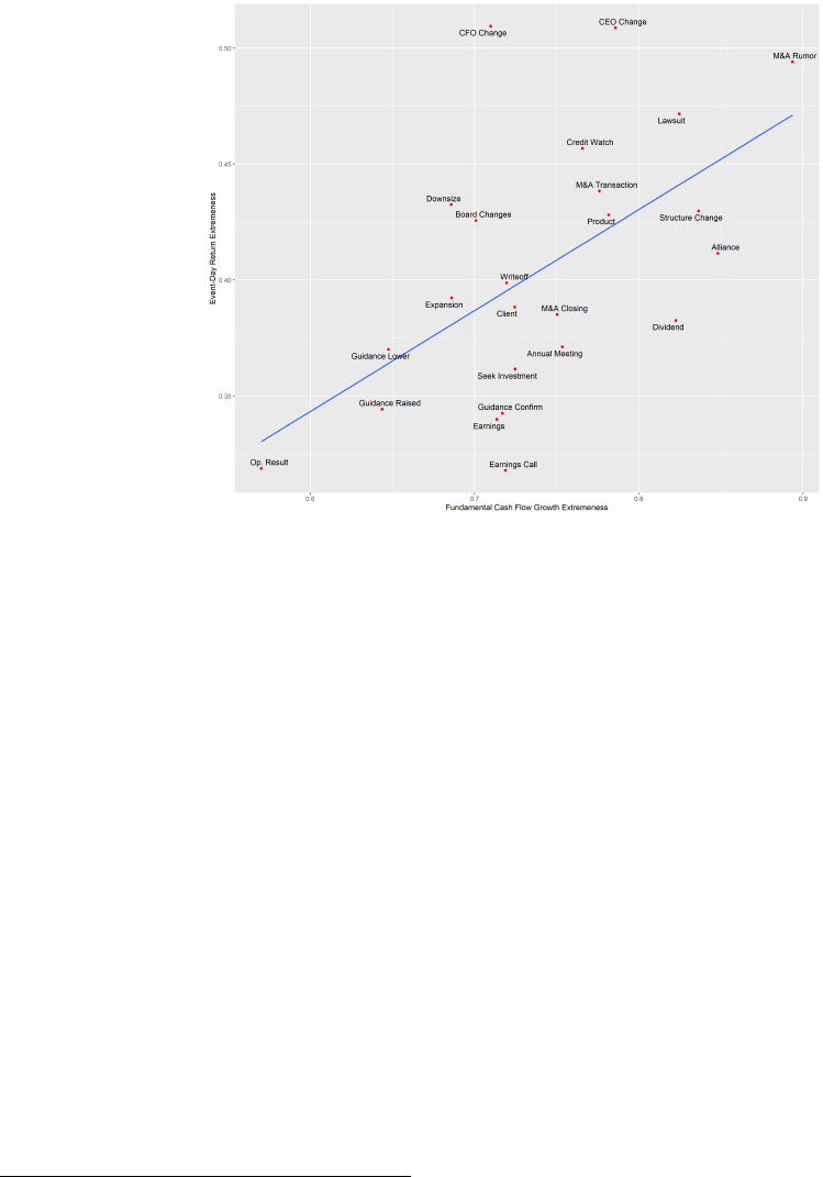
Figure 8: Extremeness of the Distribution of Fundamentals vs. Extremeness of the Distri-

bution of Event-Day Returns

Note: Figure 8 plots the relationship between the extremeness of the distribution of funda-

mentals, as proxied by the cash ﬂow growth over a 2-year horizon after the event, and the

extremeness of the distribution of event-day returns, across event types. Extremeness of the

distributions are calculated following the power-law regression speciﬁcations in eq. (14).

mean ratios (e.g. E[θ|θ > C]/E[θ|θ > 0]). As a robustness check, we report in Figure A4

the 1%/50% quantile-ratio of each event type and verify that it is highly correlated with the

fatness of the tail ζ

e

. We also compute the skew as an alternative measure and ﬁnd that

skew is also highly correlated with ζ

e

.

24

On the other hand, our measure of extremeness is distinct from other potentially intuitive

measures, such as variance or the absolute frequency of big events. What drives overreac-

tion in our model is that more extreme outliers become more representative in light of news

and subjectively overrepresented relative to other outcomes. If outcomes become uniformly

24

One major drawback of skew, however, is that higher-order moments such as skew or kurtosis cannot be

reliably measured for fat-tailed distributions.

34

bigger, all outcomes become equally more representative, which results in no distortion.

Earnings announcements provide an illustrative example. While earnings announcements

tend to be quite signiﬁcant, with relatively frequent large event-day returns, they are among

the least extreme evenypes in our sample. An outstanding earnings announcement is simply

not so big relative to other signiﬁcant earnings announcements, and thus earnings announce-

ments are not diagnostic of extreme fundamentals. Empirically, we conﬁrm in Section 5.1.2

that these alternative measures do not predict investor reaction whereas extremeness does.

5 Extremeness and Under- and Overreaction

In the previous section, we documented signiﬁcant heterogeneity in the short-term market

reaction and the extremeness of the fundamental impact across a wide range of corporate

developments. We now turn to the key asset pricing implications of our model as outlined

in Section 2: more extreme event-types are associated with greater overreaction, reversals,

and trading volume. We document evidence consistent with these predictions and test and

rule out several alternative explanations of these results.

5.1 Prediction 1: Overreaction and Extremeness

We test Prediction 1 by comparing the fatness of the tail of each type of corporate events,

ζ

e

against its degree of post-announcement drift or reversal.

We ﬁrst present our main result in a scatterplot in Figure 9. The ﬁgure illustrates a

striking relationship between extremeness ζ

e

and the post-announcement drift/reversal β

e

across event types: fatter-tailed event types have more reversal; thinner-tailed events have

more drift. The correlation coeﬃcient is −0.59 and is statistically signiﬁcant at the 1% level.

Additionally, the estimated relationship implies close to no drift or reversals for the reference

distribution (No-Events), which has an extremeness parameter 0.35. This is consistent with

35

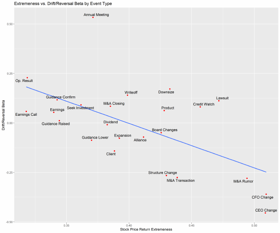
Figure 9: Post-Announcement Price Drift/Reversal vs. Extremeness

Note: Figure 9 plots the relationship between extremeness and post-announcement

drift/reversal β

e

for each event type e. Extremeness is the inverse power-law index ζ

e

esti-

mated following eq. (14), and drift/reversal β

e

is estimated following eq. (9).

our model presented in Section 2, which predicts that relative to the no news distribution,

events with less extreme fundamental distributions are more likely to have under-reaction

and that events with more extreme fundamental distributions are more likely to have over-

reaction.

Next, we estimate the relationship in a regression speciﬁcation as follows:

r

e,c,t+1,t+k

= α + β

0

· r

e,c,t,t+1

+ γ · ζ

e,t

· r

e,c,t,t+1

+ 

e,c,t

. (15)

Observations are at the corporate event level. r

e,c,t+1,t+k

is the cumulative stock price return

for a corporate event e for company c from date t + 1 to t + k, where days are restricted to

trading days. r

e,c,t,t+1

is the event-day stock return for event e of company c. γ, the coeﬃcient

of interest, captures the correlation between the future drift/reversal and the extremeness

36

of each event type. To ensure that our extremeness measurements are not contaminated by

future event returns, we estimate ζ

e

both over the entire sample period as well as using a

trailing window of three years, for which we exclude the ﬁrst three years of the sample to

ensure we have full three-year windows of returns.

25

Table 3 reports the results corresponding to eq. (15). In each speciﬁcation, we estimate a

negative and statistically signiﬁcant γ coeﬃcient. For reference, the time-varying ζ

e,t

measure

ranges from 0.19 to 1.22 (sd = 0.08), while the ﬁxed ζ

e,t

measure ranges from 0.32 to 0.51

(sd = 0.05).

26

In column (2), the estimated β coeﬃcients imply that the diﬀerences in the

tail-fatness can explain the range of post-announcement stock price movements from drifts

of 10% (= −1.28 × 0.32 + 0.51) to reversals of 14% (= −1.28 × 0.51 + 0.51). This ﬁnding is

consistent with our core prediction that more extreme event types (with higher ζ

e

) are more

overreacted to (with more negative β

e

).

5.1.1 Robustness exercises

In this section, we report results on several robustness exercises related to Prediction 1.

A. Reverse causality

One potential concern is that our results are driven by reverse causality. For example,

there may be a general force for overreaction unrelated to our mechanism, which causes the

event-day return distribution to be extreme. We address this concern using our alternative

measures of fundamental extremeness unrelated to the event-day return, by using the ex-

tremeness of the cash ﬂow growth distribution, or the long-run return distribution. If these

alternative measures of extremeness of fundamentals also predict reversals, then it is unlikely

that our results are driven by reverse causality.

We deﬁne the k-year cash ﬂow growth subsequent to each corporate news event experi-

25

As with our baseline results in Section 3, we use a 90-day horizon, and show that we obtain quantitatively

similar results with diﬀerent horizons in the Appendix (Tables A8 and A9).

26

Note that ζ < 1 for a proper distribution. In our estimates, ζ ≥ 1 for only 0.2% of rolling windows in

our sample.

37

enced by ﬁrm i in year t as ∆EP S

i,t+k

= EP S

i,t−1+k

/EP S

i,t−1

− 1, which is the percentage

change in earnings per share of ﬁrm i from the ﬁscal year immediately preceding the event

to k years later. We use horizons of 1 to 5 years subsequent to the events.

27

For our long-run

return distribution, we use the distribution of the cumulative returns up to 100 days after

the event. We estimate the extremeness of each of these distributions for each event type

following eq. (14), where we replace the event-day returns with the cash ﬂow growths and

long-run returns, respectively. These alternative estimates are based on the same sample as

the extremeness estimated on the event-day return distribution, and are similarly precise.

We repeat our analysis in eq. (15) with the extremeness of cash ﬂow growths and long-run

returns instead of the extremeness of the event-day returns as the explanatory variable:

r

e,c,t+1,t+k

= α + β

0

· r

e,c,t,t+1

+ γ · ζ

F,e

· r

e,c,t,t+1

+ 

e,c,t

, (16)

where ζ

F,e

is the extremeness of the cash ﬂow growths and long-run returns, respectively. Ta-

ble A10 reports the estimates. We estimate a negative γ coeﬃcient for each of the alternative

measures of extremeness of fundamentals. As such, the analysis using alternative measures

of fundamentals suggests that our results are not driven by reverse causality. However, as

discussed in Section 4.2, these alternative measures are computed over longer horizons and

potentially incorporate changes in stock prices due to other news, which is why we use the

event-day return distribution as the main measure of extremeness.

B. Generated regressor problem

The empirical estimation of ζ

e

coeﬃcients poses a generated regressor problem (Pagan

(1984) and Murphy and Topel (2002)) in the estimation of eq. (15). To address this, we

use the block bootstrap procedure (Politis and Romano (1994)). We draw 100 bootstrap

samples and estimate the γ coeﬃcient on each bootstrap sample following eq. (15). Figure

27

To avoid dividing by quantities close to zero, we estimate our cash ﬂow growth measure based on ﬁrms

with earnings per share in year t − 1 of at least 10 cents.

38

A5 presents the density plot of the γ estimates from the bootstrap samples. The mean is

−1.10 and the empirical 95% interval is [−2.22, −0.05], which is quantitatively in line with

the estimated γ coeﬃcients reported in Table 3. As such, our estimation of the γ coeﬃcient

in eq. (15) is quantitatively unchanged when we account for the generated regressor.

5.1.2 Testing alternative explanations

In the following section, we test alternative hypotheses that could explain the cross-sectional

variation in post-announcement drifts and reversals.

Our main econometric speciﬁcation follows eq. (15) and includes additional explana-

tory variables corresponding to each alternative hypothesis. We individually test whether

each additional variable is either quantitatively meaningful or are statistically signiﬁcant

predictors of the variation in post-announcement drift and reversal beyond our extremeness

measure ζ

e

:

r

e,c,t+1,t+k

= α + β · r

e,c,t,t+1

+ γ · ζ

e,t

· r

e,c,t,t+1

+ φ · X

e,c,t

· r

e,c,t,t+1

+ 

e,c,t

. (17)

Observations are at the event level as in eq. (15). X

e,c,t

denotes the additional explanatory

variable of interest, with φ measuring whether the additional explanatory variable can explain

the cross-sectional variation in post-announcement drift and reversal beyond extremeness ζ

e

.

We report the results of this exercise using time-varying ζ

e,t

estimates and also ﬁnd that all

results are unchanged using ζ

e

’s estimated over the full sample.

A. Familiarity with events

Investors may react diﬀerently to diﬀerent event types because they may be more accus-

tomed to some event types than others. For instance, investors may be very familiar with

earnings announcements as they are frequent and regular, whereas investors may not know

how to react when the CEO gets ﬁred because they are unfamiliar with CEO ﬁrings. To

address this concern, we compute the number of times an event of each type has occurred

39

N

e,t

as a proxy for investors’ familiarity, and estimate eq. (17) with X

e,c,t

= N

e,t

.

B. Lower-order moments of stock returns

The variation in investor reaction to news may alternatively be driven by the mean or

variance of fundamentals, rather than its extremeness. For example, if investors mechanically

overreact to event types with big returns, then diﬀerences in event-day return variance may

instead drive variations in post-announcement drift or reversal. In a similar vein, if investors

react diﬀerently to good and bad news, diﬀerences in the mean returns across diﬀerent event

types could instead generate the observed variation. To test these alternative hypotheses,

we compute the mean µ

e,t

and the variance V ar

e,t

of event-day returns for each type of

corporate events„ and estimate eq. (17) with X

t

= µ

e,t

and V ar

e,t

respectively.

C. Price impact

We also revisit our analysis in 4.1.2: the diﬀerences in post-announcement drift or re-

versal may be generated by unconditional reversal for events with larger event-day returns,

regardless of the event type. To test this explanation, we add a term that is the event-day

return, X

e,c,t

= |r|

e,c,t,t+1

.

D. Event Predictability

Another alternative explanation could be that certain types of events in the sample

are either regularly occurring or are predictable in when they occur, and that the mar-

ket reacts diﬀerently to predictable events.

28

To test this, we identify the event types

that regularly occur for a ﬁrm (i.e. operating results, earnings announcements, guidances,

dividends, earnings calls, and annual general meetings), and add the indicator variable

X

e,c,t

= 1(e is Predictable).

E. Ambiguity or noise of the news

Finally, investors may overreact to event types that have less informative signals, and

underreact to those that are more informative. To test this alternative hypothesis, we proxy

28

For example, Hartzmark and Solomon (2018) document overreaction to predictable components of earn-

ings.

40

for the ambiguity or noisiness of an event type with its average trading volume holding ﬁxed

fundamentals; if the news contains more noise, then disagreement-driven trading is likely

to be higher. We thus add a term that is the average conditional turnover, X

e,c,t

= T

e

, for

a 10% absolute event-day return. T

e

for each event type e is estimated from the following

regression:

T urnover

e,c,t

= α + β · |r

e,c,t,t+1

| + 

c,t

, (18)

where T urnover

e,c,t

is the event-day turnover of ﬁrm c experiencing an event type e on date

t, and |r

e,c,t,t+1

| is the absolute event-day return. T

e

is then α+β · 10%, or the ﬁtted turnover

for a 10% absolute event-day return for each event type e.

5.1.3 Testing for alternative hypotheses

We test all of the above alternative explanations by estimating eq. (17) by setting X

e,c,t

as

each of the alternative explanatory variables. Table 4 reports the corresponding estimates.

We ﬁnd that with the exception of ambiguity, the estimated coeﬃcients φ for none of the

alternative explanatory variables are economically and statistically signiﬁcant, whereas the

coeﬃcient corresponding to extremeness ζ

e

, γ, is negative and both economically and statis-

tically signiﬁcant for all speciﬁcations. While we ﬁnd a signiﬁcant coeﬃcient for conditional

turnover, which is our proxy for ambiguity, this is consistent with our model and empiri-

cal evidence in Section 5.2, which predicts greater trading volume for more extreme event

types. Furthermore, the coeﬃcient of our main explanatory variable ζ

e

is still signiﬁcant and

similar in magnitude. Overall, the evidence suggests that the alternative explanations are

unlikely to be driving our ﬁndings, and that extremeness is indeed a key variable driving the

cross-section of investor reaction to news.

41

5.2 Prediction 2: Volume and Extremeness

We next test Prediction 2, the relationship between extremeness and trading volume. Our

model implies that more extreme event types trigger greater disagreement between those

who receive high private signals and those who do not. Therefore, events with more extreme

return distributions should generate more trading conditional on the same fundamentals.

We measure trading volume as the turnover, deﬁned as the number of shares traded times

the share price divided by total market cap. We take two approaches to measure trading

volume conditional on the fundamentals. First, we compute the event-day turnover for each

event type conditional on the event-day returns, which is a proxy for the magnitude of the

fundamental news. For each event type, we estimate a conditional turnover, T urnover

e,10

,

for an event of each type with a 10% absolute event-day return. We then examine how

T urnover

e,10

correlates with extremeness ζ

e

across event types.

Second, we estimate the relationship between trading volume and extremeness in a panel

regression and control for the absolute value of the event-day return as a proxy for the

fundamentals of each event. The regression speciﬁcation mirrors eq. (15) and is as follows:

T urnover

e,c,t

= α + β · |r

e,c,t,t+1

| + δ · |r

e,c,t,t+1

| · ζ

e,t

+ µ

t

+ µ

e

+ 

e,c,t

, (19)

where observations are at the individual event level, T urnover

e,c,t

is the event-day turnover

for the stock of ﬁrm c that occurred at date t, r

e,c,t,t+1

is the associated event-day return,

and ζ

e,t

is the return extremeness for each event type as deﬁned before. We also include

µ

t

and µ

e

as trading day and event type ﬁxed eﬀects. Finally, δ, the coeﬃcient of interest,

measures the impact of the tail on the conditional turnover.

Figure 10 plots the relationship between extremeness ζ

e

and the conditional turnover

T urnover

e,10

, which ranges from 4.6% to 7.0%. The correlation coeﬃcient is 0.56 (p-value <

0.01). Consistent with Prediction 2, event types with fatter tails are associated with higher

turnovers conditional on the absolute event-day return. Table 5 presents the estimated coef-

42

Figure 10: Volume and Extremeness

Note: Figure 10 plots the relationship between extremeness and conditional turnover

T urnover

e,10

for each event type e. Extremeness is the inverse power-law index ζ

e

esti-

mated following eq. (14) and conditional turnover T urnover

e,10

is estimated following eq.

(19).

ﬁcients of our second approach. In each speciﬁcation, we estimate a positive and statistically

signiﬁcant δ coeﬃcient, indicating that events with fatter-tailed returns generate higher trad-

ing volume. An increase in the extremeness of the fundamental distribution from 0.32 to

0.51, i.e. from the least extreme to the most extreme fundamental distributions, corresponds

to a 1.5% increase (= 0.81 × (0.51 − 0.32) × 10) in the predicted turnover

\

T urnover

e,10

. Our

results thus suggest that extremeness ζ

e

can quantitatively explain the observed diﬀerences

in average trading volume across event types.

29

The variation in trading volume we document across event types is the trading volume holding ﬁxed

the event-day returns. The relationship between volume and the extremeness of the underlying event-day

returns is therefore not mechanically driven by diﬀerences in the magnitudes of returns.

43

5.3 Under-overreaction in Expectations Data

Having documented evidence of under-overreaction according to extremeness in stock price

and trading volume data, we now validate our theory directly using expectations data. We

proxy for investor expectations using the analyst earnings per share (EPS) forecasts reported

in I/B/E/S. Following Bouchaud et al. (2019) and Bordalo et al. (2019), we measure the

consensus I/B/E/S analyst EPS forecasts before and after corporate news events. First, to

remove stale forecasts, we only use analyst forecasts that were issued 90 days or less before

the event and revised 45 days or less after the event. Second, we winsorize the forecasts at

the 5% level to remove anomalous forecasts. Third, we focus on EPS forecasts made for two

years ahead.

30

Finally, we normalize the EPS forecasts by the price of the stock P

c,t

at the

time of the forecasts.

31

The change in consensus EPS forecast is deﬁned as the diﬀerence

between pre-event consensus EPS and post-event consensus EPS:

E

Agg

pre

[EP S

e,c,t

] =

1

N

X

a=1

E

a

pre

[EP S

e,c,t

]

E

Agg

post

[EP S

e,c,t

] =

1

N

X

a=1

E

a

post

[EP S

e,c,t

]

F orecastRevision

e,c,t

= E

Agg

post

[EP S

e,c,t

] − E

Agg

pre

[EP S

e,c,t

]

F orecastError

e,c,t

= EP S

e,c,t

− E

Agg

post

[EPS

e,c,t

],

where a is the analyst, N the number of analysts, and pre/post denoting whether the forecast

was made before or after the event.

32

To quantify the degree of belief reaction to the news, we follow Coibion and Gorod-

30

The results are qualitatively similar if we use diﬀerent forecast horizons.

31

Bouchaud et al. (2019) denote this normalized statistic as a proﬁtability measure, and refer to the

predictability of forecast errors as a proﬁtability puzzle.

32

As always, e is the event type, c the company, and t the time of the event.

44

nichenko (2015) by regressing forecast errors on forecast revisions:

F orecastError

e,c,t

= β

CG

e

· F orecastRevision

e,c,t

+ 

e,c,t

.

A negative β

CG

e

implies overreaction, in which forecasts overshoot the rational benchmark,

and conversely a positive β

CG

e

suggests underreaction. For each event type e, we estimate a

separate β

CG

e

, and then compare the estimated β

CG

e

against the extremeness measure ζ

e

.

Figure A7 in the Online Appendix plots the relationship between the two variables.

First, consensus beliefs exhibit underreaction to many event types in our sample. This is

consistent with the ﬁndings of Coibion and Gorodnichenko (2015), Bordalo et al. (2020b),

and Bouchaud et al. (2019), who ﬁnd overall underreaction to news at the consensus-level in

macroeconomic and analyst forecasts, which could be attributable to dispersed information,

general sluggishness, or analyst incentives. Second, conditional on general underreaction, we

ﬁnd that more extreme event types have less underreaction or more overreaction in beliefs,

with a correlation coeﬃcient of −0.36 (p = 0.08), which is consistent with our hypothesis

that diagnostic investors overreact more to news with more extreme distributions. In general,

we are able to move beyond market prices and trading volume and use expectations data

to ﬁnd suggestive evidence that consensus forecasts react more sensitively to more extreme

event types.

5.4 Calibration

To assess the explanatory power of our model, we perform a simple calibration exercise. Our

key parameters are the diagnostic parameter θ and the investor demand elasticity κ. We

ﬁt these parameters separately by estimating θ on returns, and then κ on trading volume.

45

Given a value of θ, we predict future stock price drift or reversals of an event by:

ˆr

e,c,t+1,t+k

= β(θ,

ˆ

ζ

e

,

ˆ

ζ

d

) · r

e,c,t,t+1

,

where β(θ,

ˆ

ζ

E

,

ˆ

ζ

d

) is given by Equation 8 and

ˆ

ζ

e

and

ˆ

ζ

d

are the estimated tail coeﬃcients. We

ﬁt θ by minimizing the prediction error,

ˆ

θ = arg min

θ

X

e,c,t

(r

e,c,t+1,t+k

− ˆr

e,c,t+1,t+k

)

2

.

and given

ˆ

θ, we estimate κ on trading volume by minimizing:

ˆκ = arg min

κ

X

e,c,t



T urnover

e,c,t

−

\

T urnover

e,c,t

(κ,

ˆ

θ, r

e,c,t,t+1

)



2

,

where

\

T urnover

e,c,t

(κ,

ˆ

θ, r

e,c,t,t+1

) is given by Equation 7.

33

Figures A8a and A8b in the Online Appendix show that our model is able to explain

the drift/reversal β

e

’s and conditional turnovers. The correlation coeﬃcients between the

calibrated and actual values are 0.65 (p < 0.01) for drift/reversal β

e

’s and 0.58 (p < 0.01)

for conditional turnovers. The ﬁnal calibrated parameters are

ˆ

θ = 0.95, ˆκ = 0.02. We also

compute the bootstrapped distribution of the diagnostic parameter θ. Figure A9 in the

Online Appendix plots the bootstrap distribution

ˆ

θ, with the 95% quantile given by [0.15,

1.62]. The range of θ is broadly consistent with previous estimates.

34

In summary, our model

is able to quantitatively ﬁt the broad cross-sectional variation in under-overreaction in prices

33

More precisely, given that the true fundamentals λ are unobservable, we instead use Equation 7 to

obtain:

d

V ol

e,c,t

=

1

2

κ · (1 + ζ

θ,E

) ·



r

e,c,t,t+1

1 + ζ

θ,e

− 1



2

34

Bordalo et al. (2020b), which focuses on macroeconomic expectations, ﬁnds θ ≈ 0.5, while Bordalo et al.

(2019), which focuses on analyst long-term forecasts, ﬁnds θ closer to 1.

46

as well as trading volume across the event types in our sample.

6 Conclusion

A large body of literature points to the existence of systematic short-term underreaction and

overreaction to news in a wide range of settings. To explain the variation in investor reac-

tions to diﬀerent types of news, we hypothesize that news that are associated with extreme

outcomes are more overreacted to, which we formalize by applying diagnostic expectations

to the setting of corporate news.

We test our hypothesis on a large dataset of corporate announcements categorized accord-

ing to their event types. We empirically document signiﬁcant heterogeneity in the short-term

market response to diﬀerent event types, as well as in the extremeness of the fundamental

distribution of these event types. We then test and conﬁrm the two key predictions of our

model: corporate event types with more extreme distributions of fundamentals are associated

with more overreaction and disagreement-driven trading volume.

While in our framework people react to news by recalling past news of the same type,

measuring precisely which events come to mind is an important area for future work. For

example, can we systematically identify which events are referenced by investors when eval-

uating new information? Why are some events referenced and not others? Understanding

which events are recalled in a given context is an important next step to understanding how

investors react to news and ultimately how information is incorporated into asset prices.

47

References

Antweiler, W. and Frank, M. Z. (2006). Do us stock markets typically overreact to corporate

news stories? Available at SSRN 878091.

Barber, B. M. and Odean, T. (2008). All that glitters: The eﬀect of attention and news

on the buying behavior of individual and institutional investors. The review of ﬁnancial

studies, 21(2):785–818.

Barberis, N., Greenwood, R., Jin, L., and Shleifer, A. (2015). X-capm: An extrapolative

capital asset pricing model. Journal of ﬁnancial economics, 115(1):1–24.

Barberis, N., Greenwood, R., Jin, L., and Shleifer, A. (2018). Extrapolation and bubbles.

Journal of Financial Economics, 129(2):203–227.

Barberis, N., Shleifer, A., and Vishny, R. (1998). A model of investor sentiment. Journal of

ﬁnancial economics, 49(3):307–343.

Bastianello, F. and Fontanier, P. (2019). Partial equilibrium thinking in general equilibrium.

Available at SSRN 3817745.

Bernard, V. L. and Thomas, J. K. (1989). Post-earnings-announcement drift: delayed price

response or risk premium? Journal of Accounting research, 27:1–36.

Bordalo, P., Coﬀman, K., Gennaioli, N., Schwerter, F., and Shleifer, A. (2020a). Memory

and representativeness. Psychological Review, 128(1):71.

Bordalo, P., Conlon, J., Gennaioli, N., Kwon, S. Y., and Shleifer, A. (2021). Memory and

probability. Working Paper.

Bordalo, P., Gennaioli, N., Ma, Y., and Shleifer, A. (2020b). Overreaction in macroeconomic

expectations. American Economic Review.

Bordalo, P., Gennaioli, N., Porta, R. L., and Shleifer, A. (2019). Diagnostic expectations

and stock returns. The Journal of Finance, 74(6):2839–2874.

Bordalo, P., Gennaioli, N., and Shleifer, A. (2018). Diagnostic expectations and credit cycles.

The Journal of Finance, 73(1):199–227.

Bouchaud, J.-P., Krueger, P., Landier, A., and Thesmar, D. (2019). Sticky expectations and

the proﬁtability anomaly. The Journal of Finance, 74(2):639–674.

Campbell, J. Y., Grossman, S. J., and Wang, J. (1993). Trading volume and serial correlation

in stock returns. The Quarterly Journal of Economics, 108(4):905–939.

48

Chan, L. K., Jegadeesh, N., and Lakonishok, J. (1996). Momentum strategies. The Journal

of Finance, 51(5):1681–1713.

Chan, W. S. (2003). Stock price reaction to news and no-news: drift and reversal after

headlines. Journal of Financial Economics, 70(2):223–260.

Chang, T. Y., Hartzmark, S. M., Solomon, D. H., and Soltes, E. F. (2017). Being surprised

by the unsurprising: Earnings seasonality and stock returns. The Review of Financial

Studies, 30(1):281–323.

Coibion, O. and Gorodnichenko, Y. (2015). Information rigidity and the expectations forma-

tion process: A simple framework and new facts. American Economic Review, 105(8):2644–

78.

Cutler, D. M., Poterba, J. M., and Summers, L. H. (1988). What moves stock prices?

Technical report, National Bureau of Economic Research.

Cutler, D. M., Poterba, J. M., and Summers, L. H. (1991). Speculative dynamics. The

Review of Economic Studies, 58(3):529–546.

Da, Z., Engelberg, J., and Gao, P. (2011). In search of attention. The Journal of Finance,

66(5):1461–1499.

Daniel, K., Hirshleifer, D., and Subrahmanyam, A. (1998). Investor psychology and security

market under-and overreactions. the Journal of Finance, 53(6):1839–1885.

Daniel, K. and Titman, S. (2006). Market reactions to tangible and intangible information.

The Journal of Finance, 61(4):1605–1643.

d’Arienzo, D. (2020). Increasing overreaction and excess volatility of long rates. Working

paper, Bocconi University.

De Bondt, W. F. and Thaler, R. (1985). Does the stock market overreact? The Journal of

ﬁnance, 40(3):793–805.

DellaVigna, S. and Pollet, J. M. (2009). Investor inattention and friday earnings announce-

ments. The Journal of Finance, 64(2):709–749.

Driscoll, J. C. and Kraay, A. C. (1998). Consistent covariance matrix estimation with

spatially dependent panel data. Review of economics and statistics, 80(4):549–560.

Duﬃe, D. (2010). Presidential address: Asset price dynamics with slow-moving capital. The

Journal of ﬁnance, 65(4):1237–1267.

49

Embrechts, P., Klüppelberg, C., and Mikosch, T. (2013). Modelling extremal events: for

insurance and ﬁnance, volume 33. Springer Science & Business Media.

Engelberg, J. (2008). Costly information processing: Evidence from earnings announcements.

In AFA 2009 San Francisco meetings paper.

Engelberg, J., Sasseville, C., and Williams, J. (2012). Market madness? the case of mad

money. Management Science, 58(2):351–364.

Enke, B., Schwerter, F., and Zimmermann, F. (2020). Associative memory and belief for-

mation. Technical report, National Bureau of Economic Research.

Eyster, E., Rabin, M., and Vayanos, D. (2019). Financial markets where traders neglect the

informational content of prices. The Journal of Finance, 74(1):371–399.

Fama, E. (1998). Market eﬃciency, long-term returns, and behavioral ﬁnance. Journal of

ﬁnancial economics, 49(3):283–306.

Gabaix, X. (2009). Power laws in economics and ﬁnance. Annu. Rev. Econ., 1(1):255–294.

Gabaix, X. (2016). Power laws in economics: An introduction. Journal of Economic Per-

spectives, 30(1):185–206.

Gabaix, X., Gopikrishnan, P., Plerou, V., and Stanley, H. E. (2003). A theory of power-law

distributions in ﬁnancial market ﬂuctuations. Nature, 423(6937):267–270.

Gabaix, X. and Ibragimov, R. (2011). Rank- 1/2: a simple way to improve the ols estimation

of tail exponents. Journal of Business & Economic Statistics, 29(1):24–39.

Giglio, S. and Kelly, B. (2018). Excess volatility: Beyond discount rates. The Quarterly

Journal of Economics, 133(1):71–127.

Graﬃn, S. D., Carpenter, M. A., and Boivie, S. (2011). What’s all that (strategic) noise?

anticipatory impression management in ceo succession. Strategic Management Journal,

32(7):748–770.

Griﬃn, D. and Tversky, A. (1992). The weighing of evidence and the determinants of

conﬁdence. Cognitive psychology, 24(3):411–435.

Hartzmark, S. M. and Shue, K. (2018). A tough act to follow: Contrast eﬀects in ﬁnancial

markets. The Journal of Finance, 73(4):1567–1613.

Hartzmark, S. M. and Solomon, D. H. (2018). Recurring ﬁrm events and predictable returns:

The within-ﬁrm time series. Annual Review of Financial Economics, 10:499–517.

50

Hong, H. and Stein, J. C. (1999). A uniﬁed theory of underreaction, momentum trading,

and overreaction in asset markets. The Journal of ﬁnance, 54(6):2143–2184.

Kahneman, D. (2011). Thinking, fast and slow. Macmillan.

Kahneman, D. and Tversky, A. (1979). Prospect Theory: An Analysis of Decision under

Risk. Econometrica, 47(2):263–291.

Knüpfer, S., Rantapuska, E., and Sarvimäki, M. (2017). Formative experiences and portfolio

choice: Evidence from the ﬁnnish great depression. The Journal of Finance, 72(1):133–166.

Kyle, A. S. (1985). Continuous auctions and insider trading. Econometrica: Journal of the

Econometric Society, pages 1315–1335.

La Porta, R. (1996). Expectations and the cross-section of stock returns. The Journal of

Finance, 51(5):1715–1742.

Lakonishok, J., Shleifer, A., and Vishny, R. W. (1994). Contrarian investment, extrapolation,

and risk. The journal of ﬁnance, 49(5):1541–1578.

Malmendier, U. and Nagel, S. (2011). Depression babies: do macroeconomic experiences

aﬀect risk taking? The Quarterly Journal of Economics, 126(1):373–416.

Murphy, K. M. and Topel, R. H. (2002). Estimation and inference in two-step econometric

models. Journal of Business & Economic Statistics, 20(1):88–97.

Nagel, S. (2012). Evaporating liquidity. The Review of Financial Studies, 25(7):2005–2039.

Nagel, S. and Xu, Z. (2019). Asset pricing with fading memory. Technical report, National

Bureau of Economic Research.

Neuhierl, A., Scherbina, A., and Schiusene, B. (2013). Market reaction to corporate press

releases. Journal of Financial and Quantitative Analysis, pages 1207–1240.

Oh, S. and Wachter, J. A. (2018). Cross-sectional skewness. Technical report, National

Bureau of Economic Research.

Pagan, A. (1984). Econometric issues in the analysis of regressions with generated regressors.

International Economic Review, pages 221–247.

Plerou, V., Gopikrishnan, P., Amaral, L. A. N., Meyer, M., and Stanley, H. E. (1999).

Scaling of the distribution of price ﬂuctuations of individual companies. Physical review

e, 60(6):6519.

51

Politis, D. N. and Romano, J. P. (1994). The stationary bootstrap. Journal of the American

Statistical association, 89(428):1303–1313.

Savor, P. G. (2012). Stock returns after major price shocks: The impact of information.

Journal of ﬁnancial Economics, 106(3):635–659.

Solomon, D. H. (2012). Selective publicity and stock prices. The Journal of Finance,

67(2):599–638.

Tetlock, P. C. (2007). Giving content to investor sentiment: The role of media in the stock

market. The Journal of ﬁnance, 62(3):1139–1168.

Tetlock, P. C. (2014). Information transmission in ﬁnance. Annu. Rev. Financ. Econ.,

6(1):365–384.

Tversky, A. and Kahneman, D. (1973). Availability: A heuristic for judging frequency and

probability. Cognitive psychology, 5(2):207–232.

Tversky, A. and Kahneman, D. (1983). Extensional versus intuitive reasoning: The conjunc-

tion fallacy in probability judgment. Psychological review, 90(4):293.

Wachter, J. A. and Kahana, M. J. (2019). A retrieved-context theory of ﬁnancial decisions.

Technical report, National Bureau of Economic Research.

Wang, C. (2019). Under- and over-reaction in yield curve expectations. Working paper,

Mendoza College of Business, University of Notre Dame.

52

7 Tables

53

Table 1: Event Summary Statistics

Event N Mean |Mean| SD Median Turnover ζ ζ(s.e.)

Alliance 3281 0.15 1.29 2.19 0.09 1.10 0.41 0.02

Annual Meeting 4109 0.05 1.20 1.79 0.05 1.03 0.37 0.01

Board Changes 21779 0.07 1.35 2.15 0.08 1.13 0.43 0.01

CEO Change 1132 0.03 2.12 3.75 0.02 2.23 0.51 0.03

CFO Change 1428 -0.07 1.66 3.20 0.05 1.80 0.51 0.04

Client 19638 0.10 1.27 2.01 0.10 1.00 0.39 0.01

Credit Watch 1323 0.28 2.38 4.00 0.10 2.26 0.46 0.03

Dividend 1093 0.14 2.37 3.59 0.19 1.86 0.38 0.02

Downsize 2823 0.02 1.57 2.75 0.04 1.46 0.43 0.02

Earnings 23561 0.13 2.59 4.01 0.12 1.99 0.34 0.00

Earnings Call 15912 0.26 3.00 4.40 0.23 2.21 0.32 0.01

Expansion 9995 0.06 1.36 2.19 0.06 1.25 0.39 0.01

Guidance Conﬁrm 19504 0.08 2.66 4.16 0.10 2.13 0.34 0.01

Guidance Lower 1172 -1.54 3.47 5.64 -0.64 2.53 0.37 0.03

Guidance Raised 2791 0.90 2.71 4.09 0.56 1.93 0.34 0.02

Lawsuit 5511 0.04 1.36 2.27 0.04 1.33 0.47 0.01

M&A Closing 11152 0.10 1.29 1.98 0.09 1.10 0.39 0.01

M&A Rumor 4796 0.34 1.65 2.87 0.13 1.44 0.49 0.02

M&A Transaction 5108 0.33 1.71 3.02 0.16 1.46 0.44 0.01

No Events 2803401 0.07 1.26 2.13 0.07 0.99 0.35 0.00

Op. Result 1454 0.00 2.37 3.38 0.00 1.97 0.32 0.03

Product 22099 0.14 1.39 2.60 0.08 1.07 0.43 0.01

Seek Investment 7880 0.15 2.01 3.20 0.09 1.50 0.36 0.01

Structure Change 2596 0.10 1.30 2.10 0.14 1.20 0.43 0.02

Writeoﬀ 3102 0.02 2.49 3.91 0.07 1.93 0.40 0.02

Note: Table 1 reports the summary statistics of event-day stock price returns and volume

for each event-type in our event dataset. The sample is all ﬁrms listed on the major US

stock exchanges with at least $2 billion in market capitalization between January 1, 2011

and December 31, 2018. |Mean| is the mean of the absolute event-day return. Mean, |Mean|,

SD, and Median are all returns measured in percentage points. Vol is the event-day trading

volume deﬁned as the number of shares traded times the share price divided by total market

capitalization times 100. ζ is the inverse power-law index corresponding to eq. (14). A

higher value of ζ corresponds to fatter tails. ζ (s.e.) is the standard error associated with

the estimation of ζ and is computed using the bootstrap method.

54

Table 2: β

e

Drift/Reversal Estimates

Event β β s.e.

Alliance -0.12 0.15

Annual Meeting 0.45 0.12

Board Changes -0.05 0.09

CEO Change -0.42 0.25

CFO Change -0.31 0.32

Client -0.18 0.08

Credit Watch 0.04 0.14

Dividend -0.05 0.06

Downsize 0.15 0.18

Earnings 0.06 0.04

Earnings Call 0.06 0.05

Expansion -0.10 0.14

Guidance Conﬁrm 0.12 0.04

Guidance Lower -0.09 0.11

Guidance Raised 0.06 0.11

Lawsuit 0.12 0.13

M&A Closing 0.05 0.08

M&A Rumor -0.29 0.16

M&A Transaction -0.28 0.08

Op. Result 0.21 0.08

Product 0.04 0.10

Seek Investment 0.13 0.06

Structure Change -0.26 0.33

Writeoﬀ 0.13 0.06

Note: Table 2 reports the β

e

drift/reversal estimates for each corporate event-type corre-

sponding to eq. (9). Standard errors are computed to account for both serial and cross-

sectional correlations in the error term.

55

Table 3: Prediction 1: Price and Extremeness

(1) (2) (3) (4)

Event-Day Return 0.56

∗∗∗

0.51

∗∗∗

0.61

∗∗∗

0.50

∗∗∗

(0.08) (0.08) (0.09) (0.08)

Event-Day Return × Tail Thickness −1.50

∗∗∗

−1.28

∗∗∗

−1.51

∗∗∗

−1.22

∗∗∗

(0.21) (0.21) (0.23) (0.23)

Constant 0.02

∗∗∗

−0.01

∗∗∗

0.01

∗∗

−0.01

∗∗∗

(0.01) (0.002) (0.01) (0.002)

Time-Varying Tails No No Yes Yes

Return Benchmark No Yes No Yes

Observations 192,525 192,525 107,915 107,915

Note: Table 3 presents the estimated results corresponding to eq. (15). Observations are

at the event level. The dependent variable is the cumulative return from day 1 to day 90

subsequent to the event. Event-Day Return is the stock price return of the ﬁrm on the day

of the event and is measured in percentage points. Tail Thickness is ζ

e,t

, the extremeness

measure given by the inverse power-law index. Time-Varying Tails indicates whether the

ζ

e,t

is computed over a rolling window (Yes) or over the entire sample (No). Return Bench-

mark indicates whether the Event-Day Return and dependent variable are abnormal returns

benchmarked against the S&P 500. Standard errors are computed to account for both serial

and cross-sectional correlations in the error term. *** p<0.01, ** p<0.05, * p<0.10.

56

Table 4: Prediction 1: Alternative Explanations

(1) (2) (3) (4) (5) (6) (7)

VARIABLES

Event-Day Return 0.57*** 0.60 0.57* 0.56*** 0.61*** 0.69** 0.92***

(0.20) (0.38) (0.34) (0.20) (0.23) (0.29) (0.27)

Event-Day Return × Tail Thickness -1.36*** -1.42** -1.37** -1.28** -1.41*** -1.62** -0.91*

(0.49) (0.67) (0.60) (0.51) (0.52) (0.66) (0.54)

Event-Day Return × Alternative Var. -7.87 -0.56 -0.064 -0.14 -2.0e-06 -0.043 -0.16*

(8.90) (5.77) (4.34) (0.16) (4.4e-06) (0.076) (0.086)

Observations 107,915 107,915 107,915 107,915 107,915 107,915 107,915

Alternative Hypothesis Mean IQR SD Abs. Sq. N Predict Ambiguity

Note: Table 4 presents the estimated results corresponding to eq. (17). Observations are

at the event level. The dependent variable is the cumulative return from day 1 to day 90

subsequent to the event. r

t

is the event-day return, or the stock price return of the ﬁrm

on the day of the event and is measured in percentage points. Tail Thickness is ζ

e,t

, the

extremeness measure given by the inverse power-law index, and is computed over rolling

windows. Alternative Var. is the explanatory regressors for alternative hypotheses. Mean is

the average event-day return. IQR is the inter-quartile range of the event-day return. SD is

the standard deviation of the event-day return. Abs. Sq. is the absolute value of the event-

day return. N is the number of total occurrences of the event. Predict is an indicator variable

for whether the occurrence of the event is predictable. Ambiguity is the average event-day

turnover of the event type conditional on the fundamentals. Returns are benchmarked to

the S&P500. Standard errors are computed to account for both serial and cross-sectional

correlations in the error term. *** p<0.01, ** p<0.05, * p<0.10.

57

Table 5: Prediction 2: Volume and Extremeness

(1) (2) (3) (4)

VARIABLES Turnover Turnover Turnover Turnover

Event-Day Return 0.31*** 0.28*** 0.23** 0.23**

(0.083) (0.083) (0.090) (0.089)

Event-Day Return × Tail Thickness 0.48** 0.59*** 0.79*** 0.81***

(0.22) (0.22) (0.25) (0.24)

Observations 192,525 192,524 192,525 192,524

R-squared 0.369 0.386 0.393 0.406

Trading Day FEs No Yes No Yes

Return Benchmark No No Yes Yes

Note: Table 5 presents the estimated results corresponding to eq. (19). Observations are at

the event level. The dependent variable is the event-day turnover, deﬁned as the volume of

shares traded times the share price divided by the market capitalization. Event-day Return

is the absolute stock price return of the ﬁrm on the day of the event and is measured in

percentage points. Tail Thickness is ζ

e,t

, the extremeness measure given by the inverse

power-law index. Return Benchmark indicates whether the Event-Day Return and the day

1 to day 90 cumulative returns are abnormal returns benchmarked against the S&P 500.

Standard errors are computed to account for both serial and cross-sectional correlations in

the error term. *** p<0.01, ** p<0.05, * p<0.10.

58

Online Appendix

Extreme events and the under-and-overreaction to news

Spencer Kwon and Johnny Tang

January 26, 2023

A Proofs

A.1 Proof of Proposition 1

First, we derive the diagnostic distribution π

θ

(λ|E, s

i

). Note:

π

d

∝ π(λ|No News) · f(s

i

= 0|λ) ∝ λ

−(ζ

−1

d

+1)

· λ

−1

This implies that the diagnostic distribution of fundamentals is given by:

π

θ

(λ|E, s

i

) ∝ π (λ|E, s

i

) ·



π (λ|E, s

i

)

π

d

(λ)



θ

∝ λ

−(ζ

−1

E

+1)

·



λ

−(ζ

−1

E

−ζ

d

)



θ

.

Setting ζ

−1

θ,E

= ζ

−1

E

+θ(ζ

−1

E

−ζ

−1

d

), the diagnostic distribution of fundamentals is given also by

the power-law distribution with tail index (1 + ζ

−1

θ,E

)

−1

. Given that the mean of a power-law

variable with scale λ

0

and tail index ζ is given by

1

1−ζ

, we obtain that the posterior diagnostic

mean is given by:

(1 + ζ

θ,E

) · max{s, λ

0,E

}, (20)

where the rational benchmark is given by:

(1 + ζ

E

) · max{s, λ

0,E

}, (21)

The Proposition follows from the observation that ζ

θ

> ζ

E

iﬀ ζ

E

> ζ

d

.

1

A.2 Proof of Proposition 2

Market clearing implies:

p

1

=

Z

λ

s=0

E

θ

[λ|s] · f(s|λ)ds

(22)

By Proposition 1, this simpliﬁes to:

p

1

= (1 + ζ

θ,E

) ·

Z

λ

0,E

0

1

λ

0,E

ds +

Z

λ

0,E

1

λ

s · ds

!

= (1 + ζ

θ,E

) ·

λ

2

0,E

+ λ

2

2λ

(23)

The expression for the rational price p

2

follows analogously, setting θ = 0.

Finally, the distribution of p

1

, as it is asymptotically linear in λ, shares the same Pareto

exponent as λ itself. To sketch out the proof, note that for X suﬃciently large, P(p

1

≥

X) ≈ P (C · λ ≥ X) ≈ D · X

−ζ

−1

.

As for volume, note that we can just compute the aggregate position of people who are

long the asset:

V ol =

Z

λ

s

∗

D

DE

(s, p

1

)ds,

(24)

where s

∗

is the signal such that the subjective expectation of fundamentals equals the market

price p

1

, or:

s

∗

=

p

1

1 + ζ

θ,E

(25)

2

Plugging this, we obtain:

V ol = κ

Z

λ

s

∗

((1 + ζ

θ,E

)s − p

1

)

1

λ

ds

=

1

2

κ(1 + ζ

θ,E

)(λ − s

∗

)

2

=

1

2

κ · (1 + ζ

θ,E

) ·



λ

2

− λ

2

0,E

2λ



2

.

(26)

Given these expressions, Proposition 2 follows from noting that ζ

θ,E

is increasing in ζ

E

,

and ζ

θ,E

> ζ

E

iﬀ ζ

E

> ζ

d

.

3

B Event Sample Selection

In this section, we describe our event sample selection criteria and provide details on the

types of corporate events in our dataset. We focus on news related to the fundamental

operations of the ﬁrm, so as discussed in Section 3, our event selection is based on two

criteria: (1) events that occurred at least 1000 times across all US companies in our sample

between 2011 and 2018 and (2) events that are not administrative, trading-related, or capital

structure changes.

There are 102 unique event types in the Capital IQ key developments dataset in our

sample. Of these, 35 event types occurred at least 1000 times across all US companies

in our sample. We list these 35 event types in Table A3. We also report in Table A3

whether each event type was included or excluded in our sample, and the reason for exclusion

(Administrative, Trading, or Capital Structure). Our ﬁnal list consists of 24 event types. As

robustness exercises, we also conduct our main analyses and test our empirical predictions

with the excluded event types added back in and ﬁnd that our results are robust to the

inclusion and exclusion of these events.

4

C Additional Robustness Exercises

C.1 Cross-section of β robustness exercises

A. Industry variations

Another potential concern is that the observed heterogeneity in post-event drift/reversal

magnitudes does not reﬂect diﬀerences in reactions to events of diﬀerent types, but to events

occurring in diﬀerent industries. To put it in extreme words, if all of our non-earnings events

happen for tech companies, it may be that the reversals we are ﬁnding reﬂect overreaction

to tech sector news, rather than diﬀerences in reactions to diﬀerent types of events.

To test this hypothesis, we estimate modiﬁed versions of eqs. (9) and (10) to include

industry-speciﬁc slopes as follows:

r

e,c,t+1,t+k

= α

e

+ β · r

e,c,t,t+1

+ β

d

· 1(Ind

d

) · r

e,c,t,t+1

+ 

e,c

r

e,c,t+1,t+k

= α

e

+ β · r

e,c,t,t+1

+ β

e

· 1(Event

e

) · r

e,c,t,t+1

+ β

d

· 1(Ind

d

) · r

e,c,t,t+1

+ 

e,c

,

(27)

where β

d

is an industry-speciﬁc slope for each industry. As such, comparing the two spec-

iﬁcations in eq. (27) tests for the diﬀerences in ﬁt of adding event-type slopes to a model

that already includes industry-speciﬁc slopes. Column (3) of Table A4 reports the estimates

corresponding to the two speciﬁcations in eq. (27) respectively. We ﬁnd that the F-test for

nested models has a test statistic of 2.63 (p-value < 0.01), which strongly rejects the industry-

speciﬁc slopes only model in favor of the model including event-type-speciﬁc slopes. This

is consistent with the idea that there is signiﬁcant variation in drifts and reversals across

event-types, even after accounting for industry variations.

B. Stability of β

e

estimates across time

Another potential concern is that the β

e

estimates at the event-level may not be stable

across time. We address this concern by re-estimating eq. (9) on two subsets of our sample

period split by time. The ﬁrst subset is all events before 2013 and the second subset is all

5

events after 2013, which approximately corresponds to splitting the number of events in our

sample in half. We use the same methodology as in eq. (9) and keep β

e

estimates with at

least 1000 observations in each subset. We then compute the correlation coeﬃcient of β

e

across all e’s. The correlation coeﬃcient is 0.53 and highly signiﬁcant (p < 0.05), which

indicates that the β

e

estimates are fairly stable but have some noise across time. Figure A3

plots the coeﬃcients across the two time periods and demonstrates the positive correlation

of the β

e

estimates across time.

C. Logarithmic vs. linear returns

A ﬁnal concern is that estimating return drifts and reversals in log returns rather than

linear returns can bias the results due to convexity. Theoretically, since the return magni-

tudes for 99% of our sample is between −0.10 and 0.10, the bias due to convexity is orders

of magnitudes smaller than the magnitudes of the returns. Nonetheless, we also estimate

the β

e

’s in linear returns corresponding to eq. (9).

Figure A2 plots the β

e

estimates for log returns and for linear returns. The linear return

β

e

’s are highly positively correlated with the log return β

e

estimates with a correlation

coeﬃcient of 0.83 (p-value < 0.01). Furthermore, the magnitudes of the dispersions in

β

e

estimates across event-types is almost identical between log returns and linear returns.

Overall, these results suggest that our main measure of drifts and reversals, β

e

, is robust to

alternative measures in absolute returns.

6

D Additional Figures and Tables

Figure A1: Reversal vs Drift β

E

’s vs. Winner-Minus-Loser Portfolios

Note: Figure A1 plots the drift/reversal β

e

coeﬃcients against the drift/reversal UMD

e

coeﬃcients for each event-type e. The β

e

coeﬃcients are estimated for each event-type

corresponding to eq. (9). The winner-minus-loser return coeﬃcients UMD

e

are estimated

for each event-type e corresponding to eq. (13).

7

Figure A2: Reversal vs Drift β

E

’s: Logarithmic Returns vs. Simple Returns

Note: Figure A1 plots the drift/reversal β

e

coeﬃcients estimated using logarithmic returns

against the drift/reversal β

e

coeﬃcients estimated using linear returns for each event-type

e. The log-return and linear-return β

e

coeﬃcients are all estimated for each event-type

corresponding to eq. (9).

8

Figure A3: Beta Estimates Across Time

Note: Figure A3 reports the drift/reversal β

e

coeﬃcients for each event-type corresponding

to eq. (9) split by time. For each event-type, we construct two sub-samples: one of all event

occurrences of the event-type before or during 2013 and one of all event occurrences of the

event-type after 2013.

9

Figure A4: Ratio of Top 1% to Top 50% vs. Tail Fatness

Note: Figure A4 plots the relationship between the ratio of the top 1% to the top 50% of

the absolute event-day stock returns against the tail fatness ζ

e

’s. The correlation coeﬃcient

is 0.78 (p-value < 0.01).

10

Figure A5: Bootstrap γ Coeﬃcients

Note: Figure A5 plots the density of γ coeﬃcients from the bootstrap test in Section 5.1.1.

The γ coeﬃcients are estimated on moving block bootstraps following eq. (15) across 1000

samples. The red dotted lines plot the 2.5% and 97.5% percentiles of the bootstrapped γ

coeﬃcients.

11

Figure A6: Extremeness vs. Post-Announcement Drift/Reversal Beta

Note: Figure A6 plots the relationship between extremeness and post-announcement

drift/reversal β

e

for each event-type e with a separate event-type for acquirers in acquisitions.

Extremeness is the inverse Pareto index ζ

e

estimated following eq. (14), and drift/reversal

β

e

is estimated following eq. (9).

12

Figure A7: Extremeness and Under-Overreaction in Beliefs

Note: Figure A7 plots extremeness of the distribution of fundamentals, as proxied by the

cash ﬂow growth over a 2-year horizon after the event, and the under-overreaction of investor

beliefs, as proxied by the Coibion and Gorodnichenko (2015) β

CG

coeﬃcient, across event

types.

13

(a) Calibration: Drift/Reversal Betas (b) Calibration: Drift/Reversal Turnover

Figure A8: Calibration: Betas and Turnover

Note: Figure A8a plots the calibrated drift/reversal β

e

’s against the actual drift/reversal

β

e

’s estimated from the data across event types. Figure A8b plots the calibrated conditional

turnovers against the actual conditional turnovers estimated from the data across event

types.

14

Figure A9: Bootstrapped Distribution of Calibrated Theta

Note: Figure A9 plots the bootstrapped distribution of calibrated θ estimates as described

in Section 5.4. We generate 100 bootstrapped draws of the data and estimate θ for each

draw. Each bootstrapped draw has the same number of observations as the original data

and is sampled with replacement.

15

Table A1: Corporate Event Sample Headlines

Event Headline

Alliance ChinaNet-Online Holdings, Inc Announces Strategic Partnership with Wuxi Jingtum

Network Technology

Annual Meeting STAAR Surgical Company, Annual General Meeting, Jun 11, 2009

Board Changes Cellectar Biosciences, Inc. Announces Board Changes

CEO Change MYOS Corporation Announces Executive Changes

CFO Change Tetraphase Pharmaceuticals, Inc. Announces Resignation of Kamalam Unninayar

as Chief Financial Oﬃcer, Eﬀective March 16, 2018

Client Ocean Power Technologies Enters Into First Commercial PB3 Agreement with Mitsui

Engineering and Shipbuilding

Credit Watch Issuer Credit Rating: BBB/Watch Neg/– From BBB/Negative/–: Local Currency

Rating

Dividend Johnson Controls International plc Approves Quarterly Cash Dividend, Payable on

Jan. 6, 2017

Downsize Pier 1 Imports Inc. Plans to Close 16 Stores

Earnings Fonar Corp. Reports Unaudited Consolidated Earnings Results for the Third Quar-

ter and Nine Months Ended March 31, 2009

Earnings Call AtriCure, Inc., Q1 2009 Earnings Call, May-05-2009

Expansion Aemetis, Inc. Completes Construction of Advanced Biodiesel Pre Treatment Unit

Required for BP Supply Agreement

Guidance Conﬁrm Pareteum Corporation Provides Revenue Guidance for the Second Quarter Ended

June 30, 2017

Guidance Lower Crestwood Revises Earnings Guidance for the Year 2016

Guidance Raised Hartford Financial Services Group Inc. Revises Earnings Guidance for the Year of

2008

Lawsuit Hospitality Properties Trust Announces Settlement of Litigation with TravelCenters

of America LLC

M&A Closing Appliance Recycling Centers of America, Inc. (NasdaqCM:ARCI) acquired GeoTraq

Inc. for $16 million.

M&A Rumor PZU Eyes AIG Assets

M&A Transaction Diﬀerential Brands Group Inc. (NasdaqCM:DFBG) entered into a deﬁnitive pur-

chase agreement to acquire majority of North American licensing business of GBG

USA, Inc. for $1.4 billion.

Op. Result Delta Air Lines, Inc. Reports Operating Results for the Quarter Ended December

2014

Product Inovio Biomedical Corporation Inﬂuenza Vaccines Demonstrate 100% Protection

Against Current Pandemic A/ H1N1 Inﬂuenza Viruses in Animal Studies

Seek Investment Insmed Seeks Acquisitions

Structure Change Diﬀusion Pharmaceuticals Inc. Approves Amendment to Certiﬁcate of Incorporation

Writeoﬀ Manitowoc Co. Inc. Announces Impairment Charges for the First Quarter of 2009

Note: Table A1 reports example news headlines for each of the corporate event-types in the

dataset.

16

Table A2: Corporate Event Overlap with Earnings Announcements

Event Closest Next Previous Day Of 5 Days Of

Alliance 30 47 48 0.12 0.10

Annual Meeting 20 22 73 0.13 0.21

Board Changes 31 44 52 0.13 0.13

CEO Change 31 49 53 0.21 0.19

CFO Change 30 45 55 0.20 0.21

Client 30 45 48 0.10 0.11

Credit Watch 31 43 55 0.18 0.14

Dividend 5 90 87 0.88 0.88

Downsize 28 47 52 0.20 0.21

Earnings 0 90 91 1.00 1.00

Earnings Call 2 90 92 0.90 0.98

Expansion 27 49 51 0.18 0.18

Guidance Conﬁrm 6 90 84 0.88 0.87

Guidance Lower 11 90 73 0.76 0.73

Guidance Raised 5 90 83 0.89 0.86

Lawsuit 31 45 50 0.11 0.10

M&A Closing 32 49 52 0.30 0.17

M&A Rumor 33 48 50 0.11 0.12

M&A Transaction 31 49 53 0.20 0.18

Op. Result 10 85 77 0.78 0.72

Product 30 44 48 0.10 0.10

Seek Investment 22 47 70 0.42 0.43

Structure Change 29 39 55 0.15 0.15

Writeoﬀ 1 91 88 0.98 0.98

Note: Table A2 reports the average proximity to earnings announcements of each corporate

event type in the database. Closest, Next, and Previous are the average numbers of days be-

tween each corporate event-type and the closest, next, and previous earnings announcement

of the same ﬁrm, respectively. Day Of and ± 5 Days Of measure the probability that events

of each corporate event-type occurred on the exact day and within 5 days of an earnings

announcement of the same ﬁrm.

17

Table A3: Event Selection Criteria

Event Included Criteria

Op. Result Included

Earnings Included

Sales and Trading Excluded Trading

Annual Meeting Included

Expansion Included

Buyback Transaction Excluded Capital Structure

Buyback Closing Excluded Capital Structure

Structure Change Included

Client Included

Guidance Lower Included

Guidance Conﬁrm Included

Guidance Raised Included

Credit Watch Included

Debt Excluded Capital Structure

Downsize Included

Dividend Included

Earnings Call Included

Earnings Release Date Excluded Administrative

Board Changes Included

CEO Change Included

CFO Change Included

Fixed Income Excluded Capital Structure

Follow-On Equity Excluded Capital Structure

Writeoﬀ Included

Index Constituents Excluded Trading

Lawsuit Included

M&A Rumor Included

M&A Transaction Included

M&A Closing Included

Private Placements Excluded Capital Structure

Product Included

Seek Investment Included

Seeking to Sell Excluded Trading

Shelf Registration Excluded Administrative

Alliance Included

Note: Table A3 reports the event types in our dataset and the inclusion/exclusion criteria

for each event type.

18

Table A4: F Tests

(1) (2)

VARIABLES

Observations 195,820 195,820

Event-Type FEs Yes Yes

Industry FEs No Yes

F1 1.79*** 1.65**

F2 1.85*** 1.70***

Note: Table A4 reports the F-statistics corresponding to testing that all event-type coef-

ﬁcients are jointly equal to zero (F1) and that all event-type coeﬃcients are jointly equal

(F2). Column (1) reports the test for coeﬃcients estimated in eq. (10). Column (2) reports

the test statistics for coeﬃcients estimated in eq. (27), i.e. with industry ﬁxed eﬀects.

19

Table A5: Firm-Day Panel

Event β β (s.e.) β β (s.e.) β β (s.e.)

Alliance 0.06 0.11 0.06 0.11 0.09 0.1

Annual Meeting 0.43 0.06 0.43 0.07 0.41 0.06

Board Changes -0.04 0.03 -0.04 0.03 -0.04 0.03

CEO Change -0.37 0.1 -0.37 0.1 -0.38 0.11

CFO Change 0.11 0.09 0.11 0.09 0.09 0.09

Client -0.14 0.07 -0.14 0.06 -0.11 0.06

Credit Watch -0.13 0.1 -0.13 0.1 -0.11 0.1

Downsize 0.01 0.13 0.01 0.13 0 0.13

Earnings 0.06 0.01 0.06 0.01 0.06 0.01

Expansion -0.04 0.06 -0.04 0.06 -0.03 0.07

Lawsuit -0.02 0.1 -0.02 0.1 -0.04 0.1

M&A Closing 0.08 0.04 0.07 0.03 0.09 0.04

M&A Rumor -0.32 0.14 -0.32 0.14 -0.26 0.14

M&A Transaction -0.15 0.03 -0.15 0.03 -0.11 0.04

Product 0.07 0.04 0.06 0.04 0.09 0.04

Seek Investment 0.06 0.03 0.06 0.02 0.07 0.02

Structure Change -0.1 0.15 -0.1 0.16 -0.11 0.16

f(r

c,t

) Baseline Linear Non-Parametric

Note: Table A5 reports the estimated results corresponding to eq. (11). f(r

c,t

) is the

function for controlling for event-day returns. Baseline indicates no f(r

c,t

) function. Linear

indicates f(r

c,t

) = γ · r

c,t

. Non-Parametric indicates f(r

c,t

) =

P

10

i=1

γ

i

· 1(r

c,t

∈ ∆

i

), where

1(r

c,t

∈ ∆

i

) is an indicator variable for whether r

c,t

is in the i-th decile of all event-day

returns. Standard errors are computed based on Driscoll and Kraay (1998) to account for

both serial and cross-sectional correlations in the error term.

20

Table A6: Alternative Horizons

Event β

e,30

β

e,30

s.e. β

e,60

β

e,60

s.e. β

e,120

β

e,120

s.e.

Alliance -0.01 0.10 0.05 0.15 0.08 0.19

Annual Meeting 0.16 0.06 0.43 0.09 0.44 0.20

Board Changes -0.05 0.04 -0.10 0.07 -0.06 0.11

CEO Change -0.26 0.15 -0.34 0.17 -0.43 0.33

CFO Change -0.14 0.14 -0.04 0.26 -0.33 0.37

Client -0.04 0.04 -0.11 0.08 -0.10 0.08

Credit Watch 0.03 0.06 0.09 0.09 0.04 0.19

Dividend 0.06 0.02 0.05 0.08 -0.10 0.06

Downsize 0.08 0.08 0.15 0.12 0.23 0.23

Earnings 0.04 0.02 0.07 0.03 0.12 0.05

Earnings Call 0.06 0.02 0.08 0.03 0.12 0.07

Expansion -0.03 0.08 -0.06 0.12 -0.07 0.14

Guidance Conﬁrm 0.05 0.02 0.10 0.03 0.17 0.05

Guidance Lower -0.09 0.05 -0.01 0.09 -0.04 0.13

Guidance Raised 0.03 0.05 0.06 0.07 0.07 0.08

Lawsuit 0.03 0.07 0.19 0.10 0.32 0.18

M&A Closing 0.08 0.05 0.08 0.08 -0.01 0.12

M&A Rumor -0.14 0.05 -0.24 0.11 -0.36 0.22

M&A Transaction 0.02 0.04 0.00 0.06 -0.31 0.10

Op. Result 0.07 0.05 0.18 0.07 0.34 0.15

Product 0.03 0.05 0.05 0.08 0.16 0.10

Seek Investment 0.03 0.03 0.08 0.04 0.23 0.06

Structure Change -0.14 0.20 0.04 0.15 -0.40 0.37

Writeoﬀ 0.05 0.04 0.13 0.06 0.21 0.06

Note: Table A6 reports the β

e

drift/reversal estimates for each corporate event-type corre-

sponding to eq. (9) for varying time horizons (30 days, 60 days, and 120 days). Standard

errors are computed to account for both serial and cross-sectional correlations in the error

term.

21

Table A7: Alternative Measures of Fundamentals

Event-Day Return 1 0.75 0.43 0.56 0.52 0.42 0.26

Long-Run Return 0.75 1 0.34 0.33 0.32 0.22 0.14

Cash Flow 1yr 0.43 0.34 1 0.58 0.57 0.65 0.67

Cash Flow 2yr 0.56 0.33 0.58 1 0.93 0.91 0.74

Cash Flow 3yr 0.52 0.32 0.57 0.93 1 0.96 0.72

Cash Flow 4yr 0.42 0.22 0.65 0.91 0.96 1 0.83

Cash Flow 5yr 0.26 0.14 0.67 0.74 0.72 0.83 1

Note: Table A7 reports the correlation coeﬃcients between the extremeness of event-day

stock price returns (ζ

e

) with alternative measures of fundamentals: (1) the extremeness of

the long-run stock price returns, deﬁned as the power law index of the distribution of the stock

price returns of each corporate news event type over a 100-day period; (2) the extremeness

of the cash ﬂow growth, deﬁned as the percentage change in earnings per share between

the respective number of years after the event and the ﬁscal year immediately preceding the

event. For instance, the k-year cash ﬂow growth associated with an event of ﬁrm i in year t is

deﬁned as ∆EP S

i,t+k

= EP S

i,t−1+k

/EP S

i,t−1

−1. The cash ﬂow growth sample is restricted

to ﬁrms whose earnings per share in the year t − 1 are at least 10 cents. Observations are at

the event-type level.

22

Table A8: Prediction 1: 30 Days

(1) (2) (3) (4)

Event-Day Return 0.35

∗∗∗

0.31

∗∗∗

0.27

∗∗∗

0.22

∗∗∗

(0.08) (0.08) (0.09) (0.08)

Event-Day Return × Tail Thickness −0.94

∗∗∗

−0.77

∗∗∗

−0.68

∗∗∗

−0.50

∗∗

(0.21) (0.21) (0.23) (0.23)

Constant 0.01 −0.003

∗

0.01 −0.004

∗∗

(0.01) (0.002) (0.01) (0.002)

Time-Varying Tails No No Yes Yes

Return Benchmark No Yes No Yes

Observations 192,525 192,525 107,915 107,915

Note: Table A8 presents the estimated results corresponding to eq. (15). Observations are

at the event level. The dependent variable is the cumulative return from day 1 to day 30

subsequent to the event. Event-Day Return is the stock price return of the ﬁrm on the day

of the event and is measured in percentage points. Tail Thickness is ζ

e,t

, the extremeness

measure given by the Pareto index. Time-Varying Tails indicates whether the ζ

e,t

is computed

over a rolling window (Yes) or over the entire sample (No). Return Benchmark indicates

whether the Event-Day Return and the day 1 to day 30 cumulative returns are abnormal

returns benchmarked against the S&P 500. Standard errors are computed to account for

both serial and cross-sectional correlations in the error term. *** p<0.01, ** p<0.05, *

p<0.10.

23

Table A9: Prediction 1: 60 Days

(1) (2) (3) (4)

Event-Day Return 0.48

∗∗∗

0.42

∗∗∗

0.40

∗∗∗

0.35

∗∗∗

(0.08) (0.08) (0.09) (0.08)

Event-Day Return × Tail Thickness −1.20

∗∗∗

−0.98

∗∗∗

−0.95

∗∗∗

−0.80

∗∗∗

(0.21) (0.21) (0.23) (0.23)

Constant 0.01

∗∗∗

−0.01

∗∗∗

0.01 −0.01

∗∗∗

(0.01) (0.002) (0.01) (0.002)

Time-Varying Tails No No Yes Yes

Return Benchmark No Yes No Yes

Observations 192,525 192,525 107,915 107,915

Note: Table A9 presents the estimated results corresponding to eq. (15). Observations are

at the event level. The dependent variable is the cumulative return from day 1 to day 60

subsequent to the event. Event-Day Return is the stock price return of the ﬁrm on the day

of the event and is measured in percentage points. Tail Thickness is ζ

e,t

, the extremeness

measure given by the Pareto index. Time-Varying Tails indicates whether the ζ

e,t

is computed

over a rolling window (Yes) or over the entire sample (No). Return Benchmark indicates

whether the Event-Day Return and the day 1 to day 60 cumulative returns are abnormal

returns benchmarked against the S&P 500. Standard errors are computed to account for

both serial and cross-sectional correlations in the error term. *** p<0.01, ** p<0.05, *

p<0.10.

24

Table A10: Prediction 1: Reverse Casusality Tests

(1) (2) (3) (4) (5) (6)

Event-Day Return 0.45

∗∗

0.95

∗∗∗

0.97

∗∗∗

0.79

∗∗∗

0.69

∗∗∗

0.34

∗

(0.22) (0.34) (0.30) (0.22) (0.23) (0.21)

Event-Day Return × Tail Thickness −1.33

∗∗

−1.22

∗∗∗

−1.27

∗∗∗

−1.00

∗∗∗

−0.81

∗∗∗

−0.38

(0.59) (0.46) (0.41) (0.29) (0.28) (0.25)

Constant 0.02 −0.01

∗

−0.01

∗

−0.01

∗

−0.01

∗

−0.01

∗

(0.02) (0.01) (0.01) (0.01) (0.01) (0.01)

Horizon 100 Days 1 Year 2 Year 3 Year 4 Year 5 Year

Measure Returns Cash Flow Cash Flow Cash Flow Cash Flow Cash Flow

Observations 192,525 192,525 192,525 192,525 192,525 192,525

Note: Table A10 presents the estimated results corresponding to eq. (16). Observations are

at the event level. The dependent variable is the cumulative abnormal return from day 1

to day 90 subsequent to the event. Event-Day Return is the abnormal stock return of the

ﬁrm on the day of the event and is measured in percentage points. Tail Thickness is the

measure of extremeness of the distributions of long-run returns or cash ﬂow growths of each

event type e. Horizon is the time period over which the extremeness of the distributions

of returns (Returns) or cash ﬂow growths (CF) is measured. Measure is the long-run stock

returns (Returns) or cash ﬂow growths (CF). The k-year cash ﬂow growth is deﬁned as

∆EP S

i,t+k

= EP S

i,t−1+k

/EP S

i,t−1

−1, which is the percentage change in earnings per share

of ﬁrm i from the ﬁscal year immediately preceding the event, t−1, to year t+k. We exclude

ﬁrms with earnings per share in year t − 1 less than 10 cents from our sample. Standard

errors are computed to account for both serial and cross-sectional correlations in the error

term. *** p<0.01, ** p<0.05, * p<0.10.

25

Table A11: Prediction 1: Price and Extremeness, Full Sample

(1) (2) (3) (4)

VARIABLES

Event-Day Return 0.38*** 0.37** 0.49*** 0.44**

(0.14) (0.16) (0.17) (0.17)

Event-Day Return × Tail Thickness -0.99*** -0.88** -1.19*** -1.03**

(0.37) (0.41) (0.40) (0.42)

Observations 236,579 236,579 131,454 131,454

Time-Varying Tails No No Yes Yes

Return Benchmark No Yes No Yes

Note: Table A11 presents the estimated results corresponding to eq. (15) for the full set

of events listed in Table A3. Observations are at the event level. The dependent variable

is the cumulative return from day 1 to day 90 subsequent to the event. Event-Day Return

is the stock price return of the ﬁrm on the day of the event and is measured in percentage

points. Tail Thickness is ζ

e,t

, the extremeness measure given by the inverse power-law index.

Time-Varying Tails indicates whether the ζ

e,t

is computed over a rolling window (Yes) or

over the entire sample (No). Return Benchmark indicates whether the Event-Day Return

and dependent variable are abnormal returns benchmarked against the S&P 500. Standard

errors are computed to account for both serial and cross-sectional correlations in the error

term. *** p<0.01, ** p<0.05, * p<0.10.

26

Table A12: Prediction 2: Volume and Extremeness, Full Sample

(1) (2) (3) (4)

VARIABLES Turnover Turnover Turnover Turnover

Event-Day Return 0.30*** 0.27*** 0.22*** 0.21***

(0.074) (0.072) (0.073) (0.074)

Event-Day Return × Tail Thickness 0.51** 0.63*** 0.83*** 0.84***

(0.20) (0.20) (0.21) (0.21)

Constant 0.0055*** 0.0052*** 0.0059*** 0.0059***

(0.00022) (0.00022) (0.00019) (0.00020)

Observations 236,580 236,579 236,580 236,579

R-squared 0.358 0.376 0.382 0.395

Trading Day FEs No Yes No Yes

Return Benchmark No No Yes Yes

Note: Table A12 presents the estimated results corresponding to eq. (19) for the full set of

events listed in Table A3. Observations are at the event level. The dependent variable is the

event-day turnover, deﬁned as the volume of shares traded times the share price divided by

the market capitalization. Event-day Return is the absolute stock price return of the ﬁrm

on the day of the event and is measured in percentage points. Tail Thickness is ζ

e,t

, the

extremeness measure given by the inverse power-law index. Return Benchmark indicates

whether the Event-Day Return and the day 1 to day 90 cumulative returns are abnormal

returns benchmarked against the S&P 500. Standard errors are computed to account for

both serial and cross-sectional correlations in the error term. *** p<0.01, ** p<0.05, *

p<0.10.

27